GIS is finally going native.
One request to your AI assistant. NativeGIS runs it on your machine over the real 3DEP lidar of a 64 km² forest, draws the maps, measures the change, and records every step so you can replay it.
This page is the result of that request. The session was scripted: tools/demo/build_demo.js makes the calls an assistant would make, with a plain-language reason beside each. It is not a chat with a language model. Every map, 3D scene and number below was made by NativeGIS in that session, and the transcript at the bottom lists all 63 calls.
hja-summary.json
hja-summary.json
hja-summary.json
gis_fire_severity_fit, this session
3.57 billion points, 1,114 tiles, one desktop
The full 2021 USGS 3DEP lidar run covers the whole HJ Andrews boundary. Each 250 m tile gets a ground model, a pit-free canopy height model, tree tops and area metrics. The maps are the tiles mosaicked, opened in NativeGIS and drawn with gis_render.
scaleout.md
hja-summary.json
hja-summary.json
hja-summary.json
hja-summary.json
scaleout.md
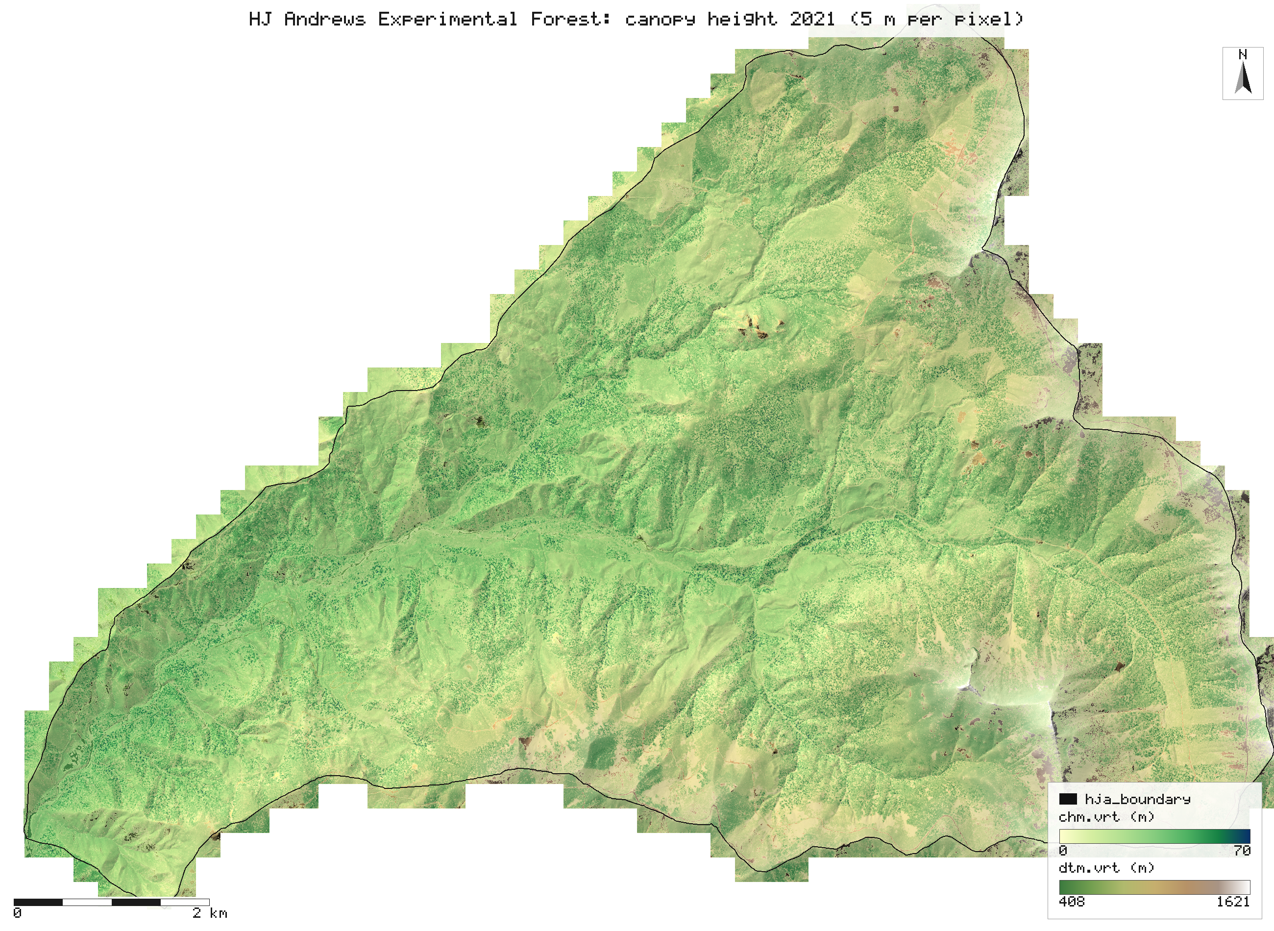
chm.vrt, dtm.vrt), which gis_open reads lazily: nothing is held at full resolution. The tiles that touch the boundary are drawn whole. Pale patches are clearcut plantations. assets/maps/forest_canopy.png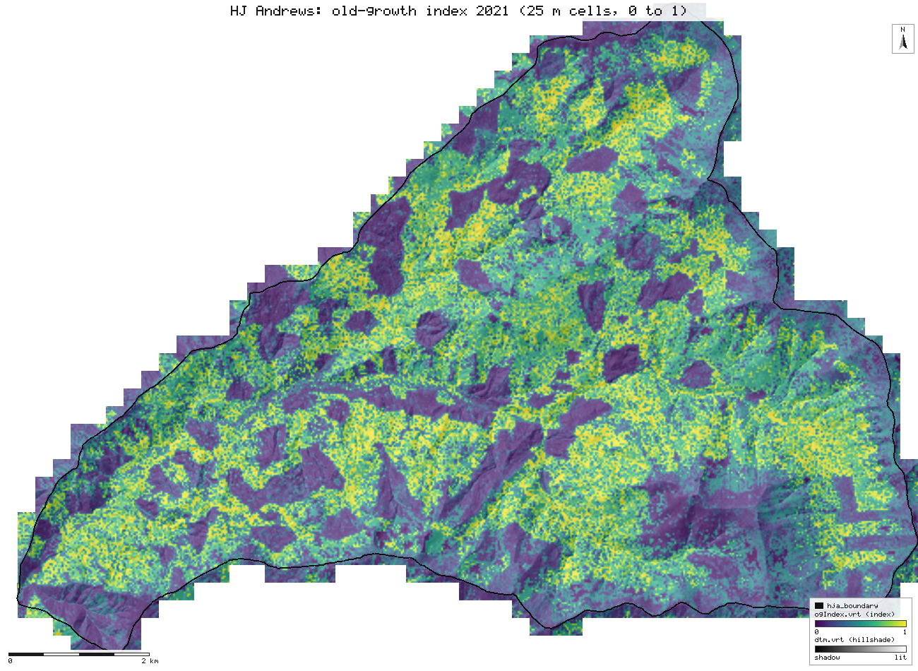
ogIndex.vrt). The weights are provisional until plot data calibrates them (ADR-2): read it as a ranking of structure, not a stand age. scaleout.md, assets/maps/forest_og.pngTrees are detected dominant and codominant tops from 5 m up. Suppressed trees under a taller crown are under-counted (7 to 22 percent of them found in the slice-1 tests), so 832,412 is not a stem count. scaleout.md
The same 56 ha in 2008 and 2021
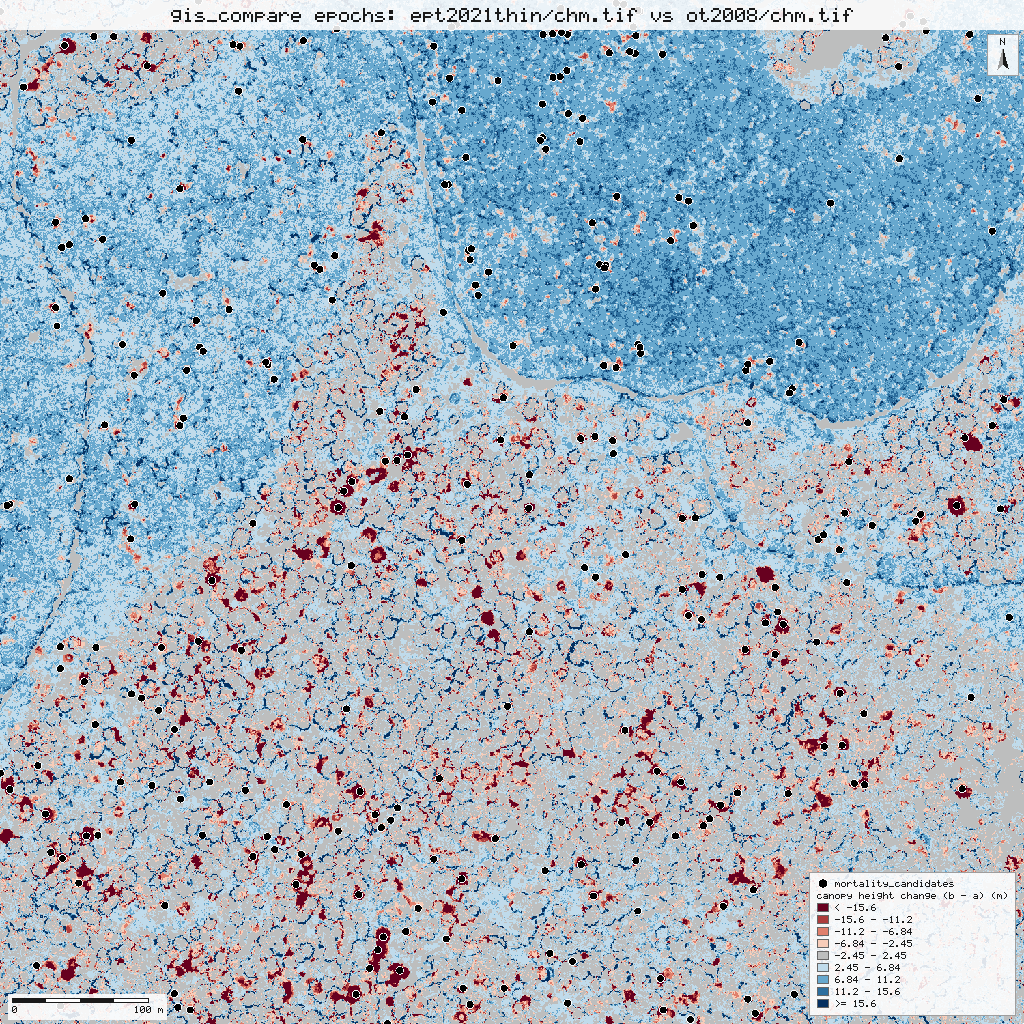
Drag the line. Both canopy height models are drawn on the same 0 to 80 m scale and extent (EPSG:26910, E 565350 to 566100, N 4900150 to 4900900). The 2021 survey is thinned to the 2008 pulse density so the two are comparable.
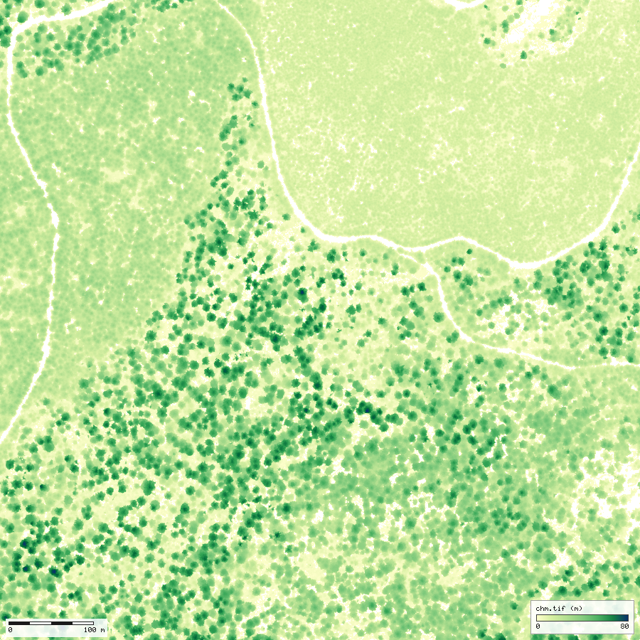
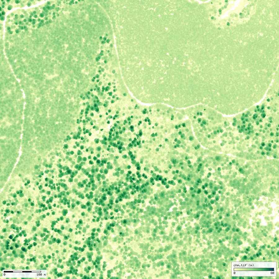
What gis_compare says (mode epochs)
- Canopy height changed by +3.47 m on average (median +3.66 m) over 2,249,993 cells.
- Canopy cover (2 m or more) went from 90.6% to 94.8%.
- 2.30 ha lost more than 10 m of height, and 0.99 ha more than 20 m.
- Trees 11,565 to 9,044; 8,051 matched (Hungarian, 2 m) and 279 mortality candidates.
- Median growth of matched trees 6.6 m over 13 years: 8.3 m for 10 to 30 m trees, 2.1 m for 30 to 50 m, 0.0 m for 50 m and over.
gis_compare epochs, this session The level of detection is 2.45 m (propagated, from 1.01 m and 0.74 m model errors). Crown expansion, mortality and harvest are not separated, and matching by position inflates the growth of small trees. compare.md
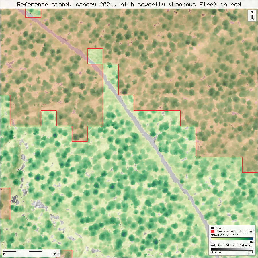
An old-growth stand in 3D, with the high-severity area laid over it
Left: the 2021 canopy surface of a 500 m reference stand, with the MTBS high-severity polygon of the 2023 Lookout Fire draped over it as a red outline and tint. Right: the 2021 point cloud of a 160 m piece across the edge of that polygon, coloured by elevation. Drag to orbit, wheel to zoom, right-drag to pan; the two cameras are linked (move one and the other follows; a checkbox in each panel unlinks it). Both are single offline HTML files written by gis_view; the polygon overlay is a small addition to that tool made for this demo.
If the panes stay dark, WebGL is off in your browser. The plan view below is the same stand drawn flat by gis_render.
How the stand was chosen
The brief was an old-growth reference stand inside or at the edge of the Lookout high-severity area. The old-growth index (ogIndex.tif, 25 m) and the MTBS dNBR6 classes (reprojected to EPSG:26910 with gis_process) were put on one grid, and every 500 m window of the lidar coverage was scored in 100 m steps (tools/demo/choose_stand.js). A window qualified when at least 98% of its cells had both layers, between 40% and 60% of its cells were class 4 (high severity), so it straddles the edge of the burned area, and its mean old-growth index was at least 0.75. Of 3,655 windows with coverage, 17 qualified, and the one with the highest mean index was taken: E 570200 to 570700, N 4897000 to 4897500, mean index 0.81, 46.5% of cells in high severity (25 m cells; the polygon measurement below uses the 30 m pixels). assets/data/stand-selection.json
- High severity covers 12.1 ha gis_process clip, measure of the 25 ha stand (48%).
- Mean old-growth index 0.81 gis_process zonal over the stand and 0.82 gis_process zonal under the high-severity part: the burned half and the rest looked alike before the fire.
- Canopy mean 29.6 m and tallest 79.3 m (1 m pit-free model from 13,536,705 points); 1,655 trees found (66.2 per ha), 482 of them 60 m or taller. gis_lidar_chm, gis_lidar_trees
A screening choice made once, not a stand inventory: no plots were measured. The 30 m severity pixels are coarser than crowns, so the outline is a stair-step, not a fire line.
Did the structure measured in 2021 predict where the Lookout Fire burned hot?
The 2023 Lookout Fire (MTBS severity, Landsat dNBR classes) overlaps 4,579 ha of the HJ Andrews lidar, 45% of the fire's mapped area slice2.md. NativeGIS area-averages the 25 m lidar layers onto the 30 m severity pixels, then summarises or fits them.
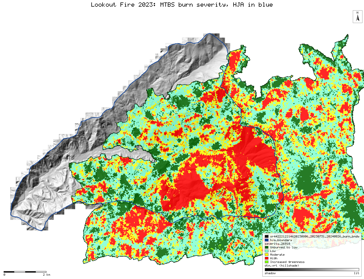
mtbs_dnbr6 legend), reprojected from Albers to UTM 10N (30 m, nearest). The HJ Andrews boundary is blue. assets/maps/fire_severity.png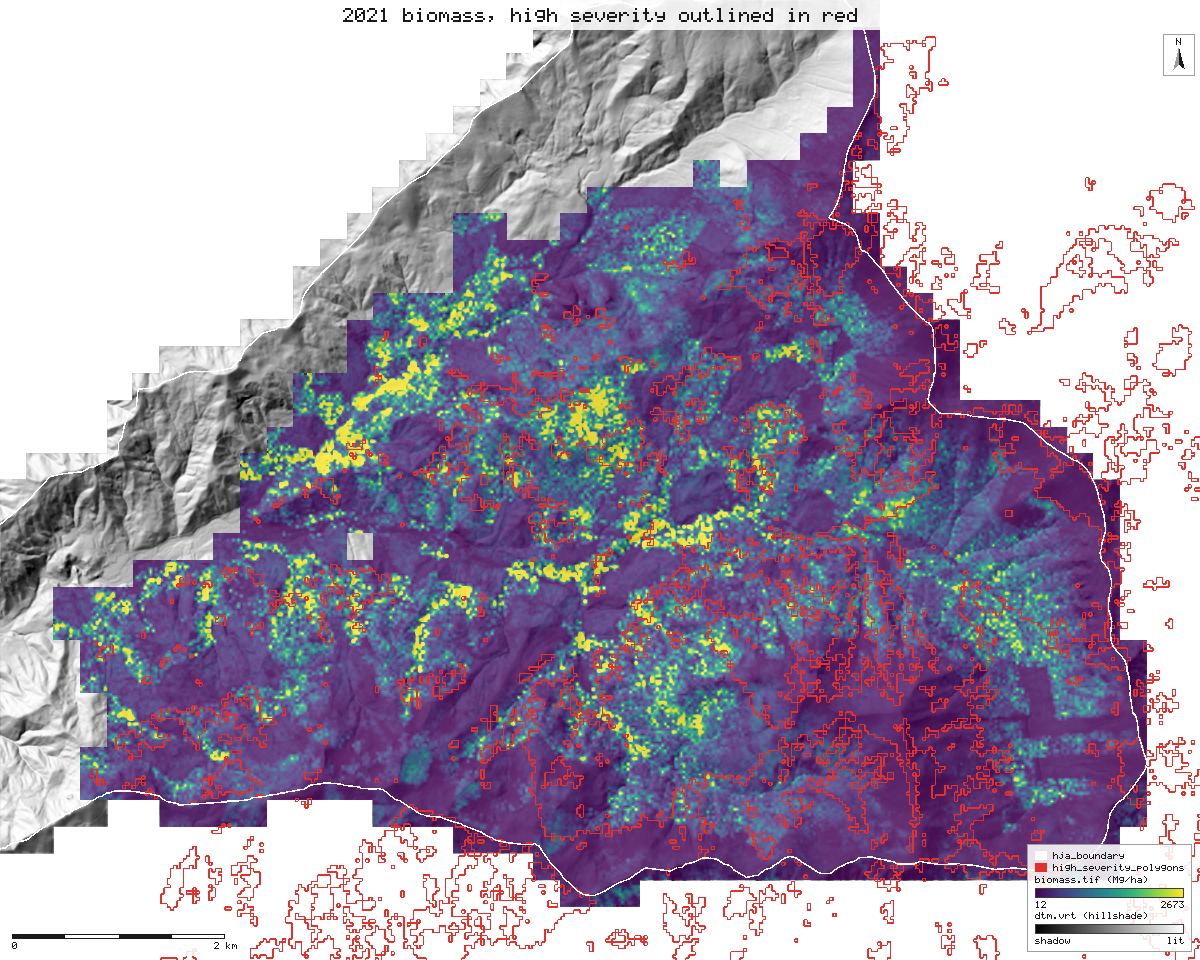
gis_process reclassify, then polygonize) outlined in red. Uncertain by tens of percent. slice2.md, assets/maps/fire_biomass.png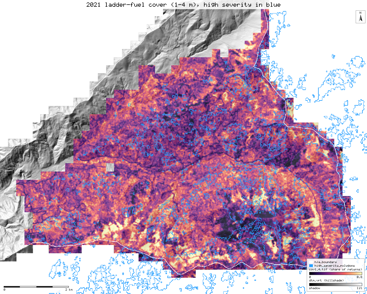
cov1_4: returns at 1 to 4 m as a share of the returns below 4 m) with high severity outlined in blue. The two do not line up. assets/maps/fire_ladder.pngPre-fire structure by severity class (30 m pixels, medians)
| MTBS class | ha with lidar | p95 height, m | canopy base, m | ladder cover, % | old-growth index | biomass Mg/ha, mean / median |
|---|---|---|---|---|---|---|
| 1 unburned to low | 714 | 32.8 | 8.2 | 44.4 | 0.19 | 327 / 226 |
| 2 low | 1,520 | 43.7 | 5.0 | 40.1 | 0.55 | 659 / 400 |
| 3 moderate | 1,057 | 44.2 | 4.2 | 40.9 | 0.58 | 610 / 392 |
| 4 high | 1,288 | 43.4 | 4.3 | 40.4 | 0.56 | 543 / 377 |
gis_fire_severity_stats, this session (assets/data/demo-results.json); equals the table in slice2.md
What this does not show
- Low, moderate and high severity burned in old forest of nearly the same structure (median old-growth index 0.55, 0.58 and 0.56). The unburned-to-low pixels are a different, shorter and younger forest.
- Burn-day weather, wind, slope and aspect, and fire progression are not in the model. That fuels explain little here does not show that fuels do not matter, and it should not be quoted that way.
- MTBS severity is a 30 m Landsat dNBR product with analyst-set thresholds, assessed about a year after the fire. It is not field burn severity and not fire behaviour. The lidar is from 2021, two years before the fire.
- The fuel models (Andersen et al. 2005, Kramer et al. 2016) are extrapolated from managed second growth to 60 to 80 m old growth and are not calibrated at HJ Andrews: treat them as indices of structure. Biomass assumes Douglas-fir everywhere.
- Pixel-level p-values are too small because neighbouring pixels are alike; the thinned fit has intervals about three times wider. slice2.md
"Lay out 40 sampling plots in Unit 12." Then: "make it 60, 100 m from roads."
Forty plots, stratified by canopy height class, off slopes over 30 percent and 50 m clear of roads, as a GeoPackage. The recipe is saved as a workflow; the second request reruns the same file with two values changed. NativeGIS names the steps those values reach (8, 10, 11, 12).
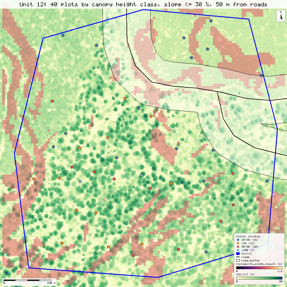
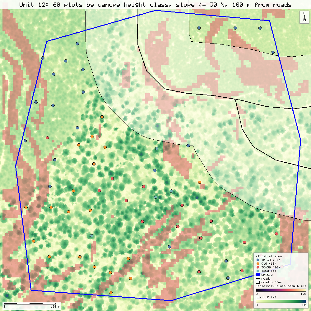
| Stratum (CHM) | feasible ha | target | achieved |
|---|---|---|---|
| <10 m | 5.04 | 12 | 12 |
| 10-30 m | 7.19 | 16 | 16 |
| 30-50 m | 4.19 | 10 | 10 |
| >=50 m | 0.89 | 2 | 2 |
| Stratum (CHM) | feasible ha | target | achieved |
|---|---|---|---|
| <10 m | 4.38 | 19 | 19 |
| 10-30 m | 4.71 | 21 | 21 |
| 30-50 m | 3.77 | 16 | 16 |
| >=50 m | 0.87 | 4 | 4 |
All 12 steps ran in 3.1 s and 4.0 s in this recording this session. The machine was shared with other jobs; the validation run measured 3.6 s and 3.3 s for the rerun generate.md. Replayed in a fresh session, the first run came back 12 identical, 0 differ, 0 failed: the GeoPackage by content and the map bit for bit generate.md.
Synthetic inputs. The samples hold no unit boundary and no road data. Unit 12 is a synthetic 26.2 ha polygon, and the roads are the forest road and its spur digitised by eye from a render of the canopy model (a few metres to about 10 m off). The sampling is real; these inputs are stand-ins. generate.md
How good is it? Compare it with something else.
Each figure below is a gis_compare call in this session, with the method named in its result. The validation recomputed them independently with numpy, scipy and shapely: 47 of 47 real-data checks agree compare.md.
| Check | Result |
|---|---|
| Ground 2008 vs 2021, RMSE over 547,600 cells | 0.228 m this session |
| Ground change beyond the 0.49 m level of detection | 1.07 ha up, 0.61 ha down this session |
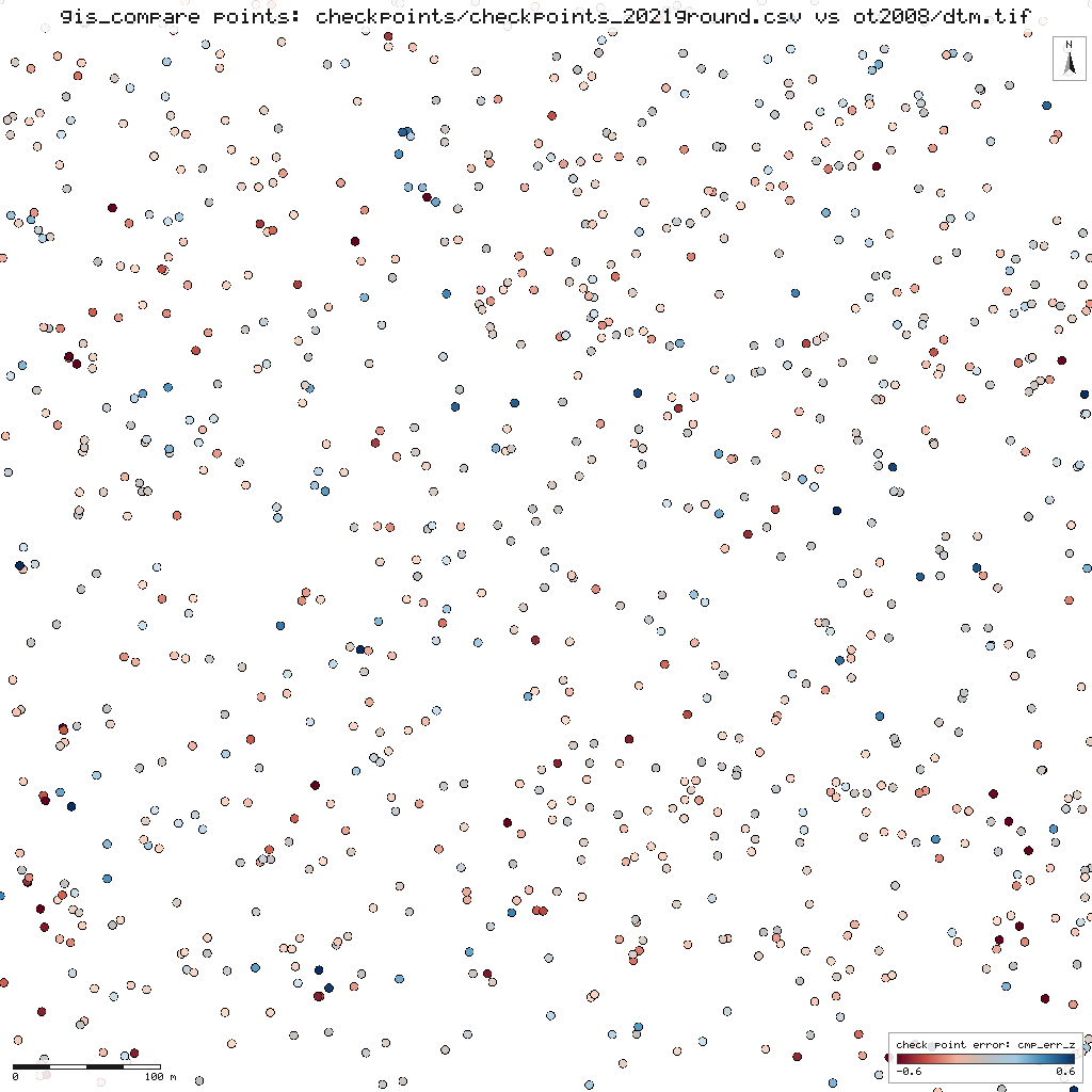
| 2008 ground vs 1,000 check points, open ground (NVA) | RMSEZ 21.0 cm, n = 74 this session |
| 2008 ground vs check points, under canopy (VVA) | RMSEZ 23.6 cm, n = 926 this session |
| Trees found vs an independent detection (2008) | omission 4.1%, commission 4.1%, F 0.959 this session |
| Canopy height model vs independent software, same ground | RMSE 1.01 m, r 0.998 slice1.md |
| Coordinate transforms vs PROJ, 18 projection pairs incl. Albers | worst 9.3e-9 m slice1.md, slice2.md |
The check points are 1,000 ground returns of the 2021 survey, so these are fit figures against another lidar survey, not a surveyed-ground accuracy class, and no class is claimed. The open-ground errors are skewed: a few large negative errors carry the RMSE (the NMAD is 6 cm). Positional accuracy follows the ASPRS Positional Accuracy Standards, Edition 2 (2023). compare.md
What was asked, and what NativeGIS did
63 calls, in order. Each shows the tool, the reason in plain language, the sentence NativeGIS answered with (it carries the key numbers), the time, and its number in the run log. The replayable record is run.json, whose steps carry the same numbers. Filter by tool:
- 1gis_open0.1 srun log step 1Open the HJ Andrews boundary (EPSG:26910).NativeGIS Opened d3a0f005_ds_1: GeoJSON with 1 layer(s): "hja_boundary" (1). CRS EPSG:26910 NAD83 / UTM zone 10N [m].
arguments
{ "path": "hja_boundary.geojson" } - 2gis_open0.1 srun log step 2Open the MTBS Lookout Fire burn-severity classes (dNBR6, Albers).NativeGIS Opened d3a0f005_ds_2: GeoTIFF 701x551, 1 band(s), uint8. CRS EPSG:5070 NAD83 / Conus Albers [m].
arguments
{ "path": "or4422212214620230806_20230731_20240826_dnbr6.tif" } - 3gis_open0.2 srun log step 3Open the ground model of the whole forest: the run's 1,114-tile mosaic (dtm.vrt, 1 m cells), read lazily.NativeGIS Opened d3a0f005_ds_3: GDAL VRT mosaic 13000x9500, 1 band(s), Float32, 1114 tile(s), read lazily by window. CRS EPSG:26910 NAD83 / UTM zone 10N [m].
arguments
{ "path": "dtm.vrt" } - 4gis_open0.1 srun log step 4Open the canopy height model of the whole forest: the 1,114-tile mosaic (chm.vrt, 0.5 m cells, 26,000 x 19,000), read lazily.NativeGIS Opened d3a0f005_ds_4: GDAL VRT mosaic 26000x19000, 1 band(s), Float32, 1114 tile(s), read lazily by window. CRS EPSG:26910 NAD83 / UTM zone 10N [m].
arguments
{ "path": "chm.vrt" } - 5gis_open0.1 srun log step 5Open the old-growth index mosaic (ogIndex.vrt, 25 m cells) from the same run.NativeGIS Opened d3a0f005_ds_5: GDAL VRT mosaic 520x380, 1 band(s), Float32, 1113 tile(s), read lazily by window. CRS EPSG:26910 NAD83 / UTM zone 10N [m].
arguments
{ "path": "ogIndex.vrt" } - 6gis_render112.2 srun log step 6Draw the forest: ground hillshade with canopy height over it.NativeGIS Wrote PNG 2600x1900 (6467570 bytes) to forest_canopy.png. PNG map 2600x1900 px in EPSG:26910 NAD83 / UTM zone 10N [m], extent x 558750 to 571750, y 4894000 to 4903500 m (13 km x 9.5 km), 5 m per pixel. Layers bottom to top: 1) ...
whole answer
Wrote PNG 2600x1900 (6467570 bytes) to forest_canopy.png. PNG map 2600x1900 px in EPSG:26910 NAD83 / UTM zone 10N [m], extent x 558750 to 571750, y 4894000 to 4903500 m (13 km x 9.5 km), 5 m per pixel. Layers bottom to top: 1) raster "dtm.vrt": terrain ramp 408 to 1621 m (minmax), hillshaded (azimuth 315°, altitude 45°, z-factor 1); values in view 405 to 1630 m, 56% of the frame covered; 2) raster "chm.vrt" at 62% opacity: chm ramp 0 to 70 m (fixed), values below 2 m transparent; values in view 0.01 to 84.5 m, 56% of the frame covered; 3) vector "hja_boundary": 1 of 1 polygon in view, fill none, outline #111111. Map furniture: title "HJ Andrews Experimental Forest: canopy height 2021 (5 m per pixel)", legend (bottom right) for 3 layer(s), scale bar 2 km (bottom left), north arrow (top right; true north 0.57° west of grid north).
arguments
{ "inline": false, "layers": [ { "handle": "ds 3", "style": { "ramp": "terrain", "hillshade": { "strength": 0.9 }, "opacity": 1 } }, { "handle": "ds 4", "style": { "ramp": "chm", "min": 0, "max": 70, "hideBelow": 2, "opacity": 0.62 } }, { "handle": "ds 1", "style": { "fill": "#00000000", "stroke": "#111111", "width": 2 } } ], "width": 2600, "height": 1900, "title": "HJ Andrews Experimental Forest: canopy height 2021 (5 m per pixel)", "outPath": "forest_canopy.png" } - 7gis_render30.1 srun log step 8Draw the old-growth index: where the structure looks like old growth.NativeGIS Wrote PNG 1300x950 (1652887 bytes) to forest_og.png. PNG map 1300x950 px in EPSG:26910 NAD83 / UTM zone 10N [m], extent x 558750 to 571750, y 4894000 to 4903500 m (13 km x 9.5 km), 10 m per pixel. Layers bottom to top: 1) raster ...
whole answer
Wrote PNG 1300x950 (1652887 bytes) to forest_og.png. PNG map 1300x950 px in EPSG:26910 NAD83 / UTM zone 10N [m], extent x 558750 to 571750, y 4894000 to 4903500 m (13 km x 9.5 km), 10 m per pixel. Layers bottom to top: 1) raster "dtm.vrt": grey hillshade (azimuth 315°, altitude 45°); values in view 405 to 1626 m, 56% of the frame covered; 2) raster "ogIndex.vrt" at 72% opacity: viridis ramp 0 to 1 index (fixed); values in view 0 to 1 index, 56% of the frame covered; 3) vector "hja_boundary": 1 of 1 polygon in view, fill none, outline #111111. Map furniture: title "HJ Andrews: old-growth index 2021 (25 m cells, 0 to 1)", legend (bottom right) for 3 layer(s), scale bar 2 km (bottom left), north arrow (top right; true north 0.57° west of grid north).
arguments
{ "inline": false, "layers": [ { "handle": "ds 3", "style": { "ramp": "none", "hillshade": { "strength": 0.9 } } }, { "handle": "ds 5", "style": { "ramp": "viridis", "min": 0, "max": 1, "opacity": 0.72, "units": "index" } }, { "handle": "ds 1", "style": { "fill": "#00000000", "stroke": "#111111", "width": 2 } } ], "width": 1300, "height": 950, "title": "HJ Andrews: old-growth index 2021 (25 m cells, 0 to 1)", "outPath": "forest_og.png" } - 8gis_info0 srun log step 10Describe the canopy mosaic (an instant answer: nothing is read from the tiles).NativeGIS d3a0f005_ds_4: raster (vrt), CRS EPSG:26910 NAD83 / UTM zone 10N [m].
arguments
{ "handle": "ds 4" } - 9gis_info0 srun log step 11Describe the old-growth index mosaic.NativeGIS d3a0f005_ds_5: raster (vrt), CRS EPSG:26910 NAD83 / UTM zone 10N [m].
arguments
{ "handle": "ds 5" } - 10gis_process2.4 srun log step 12Bring the burn-severity raster into the forest's UTM zone (30 m cells, nearest) so it lines up with the lidar.NativeGIS reproject: 830x724 raster at 30.0044094285 m, 114025 valid cells, values 1 to 5. New dataset d3a0f005_ds_6. CRS EPSG:26910 NAD83 / UTM zone 10N [m].
arguments
{ "op": "reproject", "inputs": [ { "handle": "ds 2" } ], "params": { "toEpsg": 26910, "resolution": 30, "method": "nearest" }, "name": "severity_26910" } - 11gis_process0.3 srun log step 13Keep only class 4, high severity.NativeGIS reclassify: 830x724 raster at 30.0044094285 m, 25858 valid cells, values 1 to 1. New dataset d3a0f005_ds_7. CRS EPSG:26910 NAD83 / UTM zone 10N [m].
arguments
{ "op": "reclassify", "inputs": [ { "handle": "ds 6" } ], "params": { "rules": [ { "equals": 4, "value": 1 } ], "other": "nodata" }, "name": "high_severity_mask" } - 12gis_process3.1 srun log step 14Turn the high-severity cells into polygons (dissolved), to lay over other layers.NativeGIS polygonize: 1 feature(s) (MultiPolygon), area 23264313.681 m2. New dataset d3a0f005_ds_8. CRS EPSG:26910 NAD83 / UTM zone 10N [m].
arguments
{ "op": "polygonize", "inputs": [ { "handle": "ds 7" } ], "params": { "dissolve": true, "field": "severity" }, "name": "high_severity_polygons" } - 13gis_process0 srun log step 15Measure the high-severity polygons.NativeGIS measure: 1 feature(s) (MultiPolygon), area 23264313.681 m2. Dry run, nothing kept. CRS EPSG:26910 NAD83 / UTM zone 10N [m].
arguments
{ "op": "measure", "inputs": [ { "handle": "ds 8" } ], "params": { "fields": [ "area" ] }, "dryRun": true } - 14gis_open0.1 srun log step 16Open the ground mosaic again for the shaded background.NativeGIS Opened d3a0f005_ds_9: GDAL VRT mosaic 13000x9500, 1 band(s), Float32, 1114 tile(s), read lazily by window. CRS EPSG:26910 NAD83 / UTM zone 10N [m].
arguments
{ "path": "dtm.vrt" } - 15gis_open0 srun log step 17Open the MTBS fire perimeter (Albers shapefile).NativeGIS Opened d3a0f005_ds_10: Shapefile with 1 layer(s): "or4422212214620230806_20230731_20240826…" (1). CRS EPSG:5070 NAD83 / Conus Albers [m].
arguments
{ "path": "or4422212214620230806_20230731_20240826_burn_bndy.shp", "epsg": 5070 } - 16gis_open0 srun log step 18Open the hmax layer from the fire/fuels run (25 m).NativeGIS Opened d3a0f005_ds_11: Cloud Optimized GeoTIFF 410x330, 1 band(s), float32. CRS EPSG:26910 NAD83 / UTM zone 10N [m].
arguments
{ "path": "hmax.tif" } - 17gis_open0 srun log step 19Open the ogIndex layer from the fire/fuels run (25 m).NativeGIS Opened d3a0f005_ds_12: Cloud Optimized GeoTIFF 410x330, 1 band(s), float32. CRS EPSG:26910 NAD83 / UTM zone 10N [m].
arguments
{ "path": "ogIndex.tif" } - 18gis_open0 srun log step 20Open the cov1_4 layer from the fire/fuels run (25 m).NativeGIS Opened d3a0f005_ds_13: Cloud Optimized GeoTIFF 410x330, 1 band(s), float32. CRS EPSG:26910 NAD83 / UTM zone 10N [m].
arguments
{ "path": "cov1_4.tif" } - 19gis_open0 srun log step 21Open the ladderCover layer from the fire/fuels run (25 m).NativeGIS Opened d3a0f005_ds_14: Cloud Optimized GeoTIFF 410x330, 1 band(s), float32. CRS EPSG:26910 NAD83 / UTM zone 10N [m].
arguments
{ "path": "ladderCover.tif" } - 20gis_open0 srun log step 22Open the cbh layer from the fire/fuels run (25 m).NativeGIS Opened d3a0f005_ds_15: Cloud Optimized GeoTIFF 410x330, 1 band(s), float32. CRS EPSG:26910 NAD83 / UTM zone 10N [m].
arguments
{ "path": "cbh.tif" } - 21gis_open0 srun log step 23Open the p95 layer from the fire/fuels run (25 m).NativeGIS Opened d3a0f005_ds_16: Cloud Optimized GeoTIFF 410x330, 1 band(s), float32. CRS EPSG:26910 NAD83 / UTM zone 10N [m].
arguments
{ "path": "p95.tif" } - 22gis_open0 srun log step 24Open the biomass layer from the fire/fuels run (25 m).NativeGIS Opened d3a0f005_ds_17: Cloud Optimized GeoTIFF 410x330, 1 band(s), float32. CRS EPSG:26910 NAD83 / UTM zone 10N [m].
arguments
{ "path": "biomass.tif" } - 23gis_render6.4 srun log step 25Draw the Lookout Fire burn severity (MTBS classes) over the ground, with the HJ Andrews boundary.NativeGIS Wrote PNG 1200x920 (469959 bytes) to fire_severity.png. PNG map 1200x920 px in EPSG:26910 NAD83 / UTM zone 10N [m], extent x 558500 to 575500, y 4891983 to 4905017 m (17 km x 13 km), 14.2 m per pixel. Layers bottom to top: 1) ...
whole answer
Wrote PNG 1200x920 (469959 bytes) to fire_severity.png. PNG map 1200x920 px in EPSG:26910 NAD83 / UTM zone 10N [m], extent x 558500 to 575500, y 4891983 to 4905017 m (17 km x 13 km), 14.2 m per pixel. Layers bottom to top: 1) raster "dtm.vrt": grey hillshade (azimuth 315°, altitude 45°); values in view 405 to 1620 m, 31% of the frame covered; 2) raster "severity_26910" at 85% opacity: named classes (class table mtbs_dnbr6): 1 Unburned to low, 2 Low, 3 Moderate, 4 High, 5 Increased greenness; values in view 1 to 5, 46% of the frame covered; 3) vector "hja_boundary": 1 of 1 polygon in view, fill none, outline #0b3d91; 4) vector "or4422212214620230806_20230731_20240826_burn_bndy" (reprojected from EPSG:5070): 1 of 1 polygon in view, fill none, outline #111111. Map furniture: title "Lookout Fire 2023: MTBS burn severity, HJA in blue", legend (bottom right) for 4 layer(s), scale bar 2 km (bottom left), north arrow (top right; true north 0.58° west of grid north).
arguments
{ "inline": false, "layers": [ { "handle": "ds 9", "style": { "ramp": "none", "hillshade": { "strength": 0.9 } } }, { "handle": "ds 6", "style": { "classes": "mtbs_dnbr6", "opacity": 0.85 } }, { "handle": "ds 1", "style": { "fill": "#00000000", "stroke": "#0b3d91", "width": 2 } }, { "handle": "ds 10", "style": { "fill": "#00000000", "stroke": "#111111", "width": 1.5 } } ], "extent": [ 558500, 4892000, 575500, 4905000 ], "width": 1200, "height": 920, "title": "Lookout Fire 2023: MTBS burn severity, HJA in blue", "outPath": "fire_severity.png" } - 24gis_render5.1 srun log step 27Draw the pre-fire biomass the lidar implies, with the high-severity polygons outlined on top.NativeGIS Wrote PNG 1200x960 (1300254 bytes) to fire_biomass.png. PNG map 1200x960 px in EPSG:26910 NAD83 / UTM zone 10N [m], extent x 561000 to 572250, y 4894000 to 4903000 m (11.3 km x 9 km), 9.38 m per pixel. Layers bottom to top: 1) ...
whole answer
Wrote PNG 1200x960 (1300254 bytes) to fire_biomass.png. PNG map 1200x960 px in EPSG:26910 NAD83 / UTM zone 10N [m], extent x 561000 to 572250, y 4894000 to 4903000 m (11.3 km x 9 km), 9.38 m per pixel. Layers bottom to top: 1) raster "dtm.vrt": grey hillshade (azimuth 315°, altitude 45°); values in view 475 to 1619 m, 62% of the frame covered; 2) raster "biomass.tif" at 80% opacity: viridis ramp 12 to 2673 Mg/ha (percentile 2-98); values in view 0 to 16968 Mg/ha, 49% of the frame covered; 3) vector "high_severity_polygons": 1 of 1 polygon in view, fill none, outline #e5312b; 4) vector "hja_boundary": 1 of 1 polygon in view, fill none, outline #ffffff. Map furniture: title "2021 biomass, high severity outlined in red", legend (bottom right) for 4 layer(s), scale bar 2 km (bottom left), north arrow (top right; true north 0.58° west of grid north).
arguments
{ "inline": false, "layers": [ { "handle": "ds 9", "style": { "ramp": "none", "hillshade": { "strength": 0.9 } } }, { "handle": "ds 17", "style": { "ramp": "viridis", "stretch": "percentile", "percentiles": [ 2, 98 ], "opacity": 0.8, "units": "Mg/ha" } }, { "handle": "ds 8", "style": { "fill": "#00000000", "stroke": "#e5312b", "width": 1.4 } }, { "handle": "ds 1", "style": { "fill": "#00000000", "stroke": "#ffffff", "width": 1.5 } } ], "extent": [ 561000, 4894000, 572250, 4903000 ], "width": 1200, "height": 960, "title": "2021 biomass, high severity outlined in red", "outPath": "fire_biomass.png" } - 25gis_render5.7 srun log step 29Draw the ladder-fuel cover (1 to 4 m) the same way, to see whether it lines up with the red.NativeGIS Wrote PNG 1200x960 (1439459 bytes) to fire_ladder.png. PNG map 1200x960 px in EPSG:26910 NAD83 / UTM zone 10N [m], extent x 561000 to 572250, y 4894000 to 4903000 m (11.3 km x 9 km), 9.38 m per pixel. Layers bottom to top: 1) ...
whole answer
Wrote PNG 1200x960 (1439459 bytes) to fire_ladder.png. PNG map 1200x960 px in EPSG:26910 NAD83 / UTM zone 10N [m], extent x 561000 to 572250, y 4894000 to 4903000 m (11.3 km x 9 km), 9.38 m per pixel. Layers bottom to top: 1) raster "dtm.vrt": grey hillshade (azimuth 315°, altitude 45°); values in view 475 to 1619 m, 62% of the frame covered; 2) raster "cov1_4.tif" at 80% opacity: magma ramp 0 to 0.8 share of returns (fixed); values in view 0 to 0.97 share of returns, 49% of the frame covered; 3) vector "high_severity_polygons": 1 of 1 polygon in view, fill none, outline #2aa1ff; 4) vector "hja_boundary": 1 of 1 polygon in view, fill none, outline #ffffff. Map furniture: title "2021 ladder-fuel cover (1-4 m), high severity in blue", legend (bottom right) for 4 layer(s), scale bar 2 km (bottom left), north arrow (top right; true north 0.58° west of grid north).
arguments
{ "inline": false, "layers": [ { "handle": "ds 9", "style": { "ramp": "none", "hillshade": { "strength": 0.9 } } }, { "handle": "ds 13", "style": { "ramp": "magma", "min": 0, "max": 0.8, "opacity": 0.8, "units": "share of returns" } }, { "handle": "ds 8", "style": { "fill": "#00000000", "stroke": "#2aa1ff", "width": 1.4 } }, { "handle": "ds 1", "style": { "fill": "#00000000", "stroke": "#ffffff", "width": 1.5 } } ], "extent": [ 561000, 4894000, 572250, 4903000 ], "width": 1200, "height": 960, "title": "2021 ladder-fuel cover (1-4 m), high severity in blue", "outPath": "fire_ladder.png" } - 26gis_fire_severity_stats3.3 srun log step 31For each severity class, summarise the lidar structure under it (30 m pixels, lidar cells area-averaged).NativeGIS 50875 MTBS pixels (4578.8 ha) have LiDAR; high severity (class 4): 1287.5 ha. Layers: 7.
arguments
{ "severity": "ds 2", "layers": { "hmax": "ds 11", "ogIndex": "ds 12", "cov1_4": "ds 13", "ladderCover": "ds 14", "cbh": "ds 15", "p95": "ds 16", "biomass": "ds 17" }, "footprint": "hmax", "percentiles": [ 10, 50, 90 ] } - 27gis_fire_severity_fit4.2 srun log step 33Fit high severity against the ladder-fuel cover alone.NativeGIS High severity (class 4) on 50873 pixels (14306 high): AUC 0.507, McFadden R2 0.001; odds ratios per sd: cov1_4 OR 0.94.
arguments
{ "severity": "ds 2", "layers": { "hmax": "ds 11", "ogIndex": "ds 12", "cov1_4": "ds 13", "ladderCover": "ds 14", "cbh": "ds 15", "p95": "ds 16", "biomass": "ds 17" }, "predictors": [ "cov1_4" ], "footprint": "hmax" } - 28gis_fire_severity_fit4.1 srun log step 35Repeat the fit on every third pixel in each direction, a check on neighbouring pixels being alike.NativeGIS High severity (class 4) on 5660 pixels (1601 high): AUC 0.507, McFadden R2 0.001; odds ratios per sd: cov1_4 OR 0.94.
arguments
{ "severity": "ds 2", "layers": { "hmax": "ds 11", "ogIndex": "ds 12", "cov1_4": "ds 13", "ladderCover": "ds 14", "cbh": "ds 15", "p95": "ds 16", "biomass": "ds 17" }, "predictors": [ "cov1_4" ], "footprint": "hmax", "thin": 3 } - 29gis_fire_severity_fit3.3 srun log step 37Fit it again with the structure measures together.NativeGIS High severity (class 4) on 50655 pixels (14295 high): AUC 0.577, McFadden R2 0.012; odds ratios per sd: cov1_4 OR 0.83, cbh OR 0.75, p95 OR 1.04.
arguments
{ "severity": "ds 2", "layers": { "hmax": "ds 11", "ogIndex": "ds 12", "cov1_4": "ds 13", "ladderCover": "ds 14", "cbh": "ds 15", "p95": "ds 16", "biomass": "ds 17" }, "predictors": [ "cov1_4", "cbh", "p95" ], "footprint": "hmax" } - 30gis_open0.3 srun log step 39Open the 2008 canopy height model of the 56 ha window.NativeGIS Opened d3a0f005_ds_18: Cloud Optimized GeoTIFF 1500x1500, 1 band(s), float32. CRS EPSG:26910 NAD83 / UTM zone 10N [m].
arguments
{ "path": "chm.tif" } - 31gis_open0.3 srun log step 40Open the 2021 canopy model, thinned to the 2008 pulse density so the two are comparable.NativeGIS Opened d3a0f005_ds_19: Cloud Optimized GeoTIFF 1500x1500, 1 band(s), float32. CRS EPSG:26910 NAD83 / UTM zone 10N [m].
arguments
{ "path": "chm.tif" } - 32gis_open0.1 srun log step 41Open the 2008 ground model.NativeGIS Opened d3a0f005_ds_20: Cloud Optimized GeoTIFF 750x750, 1 band(s), float32. CRS EPSG:26910 NAD83 / UTM zone 10N [m].
arguments
{ "path": "dtm.tif" } - 33gis_open0.1 srun log step 42Open the 2021 ground model, thinned like the canopy model.NativeGIS Opened d3a0f005_ds_21: Cloud Optimized GeoTIFF 750x750, 1 band(s), float32. CRS EPSG:26910 NAD83 / UTM zone 10N [m].
arguments
{ "path": "dtm.tif" } - 34gis_open0.1 srun log step 43Open the full-density 2021 ground model (for the ground comparison, as in docs/validation/compare.md).NativeGIS Opened d3a0f005_ds_22: Cloud Optimized GeoTIFF 750x750, 1 band(s), float32. CRS EPSG:26910 NAD83 / UTM zone 10N [m].
arguments
{ "path": "dtm.tif" } - 35gis_open0.1 srun log step 44Open the 2008 tree tops.NativeGIS Opened d3a0f005_ds_23: GeoJSON with 1 layer(s): "trees" (11565). CRS EPSG:26910 NAD83 / UTM zone 10N [m].
arguments
{ "path": "trees.geojson" } - 36gis_open0.1 srun log step 45Open the 2021 tree tops.NativeGIS Opened d3a0f005_ds_24: GeoJSON with 1 layer(s): "trees" (9044). CRS EPSG:26910 NAD83 / UTM zone 10N [m].
arguments
{ "path": "trees.geojson" } - 37gis_render1 srun log step 46Draw the 2008 canopy.NativeGIS Wrote PNG 900x900 (1356852 bytes) to canopy_2008.png. PNG map 900x900 px in EPSG:26910 NAD83 / UTM zone 10N [m], extent x 565350 to 566100, y 4900150 to 4900900 m (750 m x 750 m), 0.83 m per pixel. Layers bottom to top: 1) raster ...
whole answer
Wrote PNG 900x900 (1356852 bytes) to canopy_2008.png. PNG map 900x900 px in EPSG:26910 NAD83 / UTM zone 10N [m], extent x 565350 to 566100, y 4900150 to 4900900 m (750 m x 750 m), 0.83 m per pixel. Layers bottom to top: 1) raster "chm.tif": chm ramp 0 to 80 m (fixed), values below 0.5 m transparent; values in view 0 to 82.9 m, 100% of the frame covered. Map furniture: legend (bottom right) for 1 layer(s), scale bar 100 m (bottom left).
arguments
{ "inline": false, "layers": [ { "handle": "ds 18", "style": { "ramp": "chm", "min": 0, "max": 80, "hideBelow": 0.5 } } ], "extent": [ 565350, 4900150, 566100, 4900900 ], "width": 900, "height": 900, "northArrow": false, "outPath": "canopy_2008.png" } - 38gis_render1.8 srun log step 47Draw the 2021 canopy on the same scale and extent.NativeGIS Wrote PNG 900x900 (1334575 bytes) to canopy_2021.png. PNG map 900x900 px in EPSG:26910 NAD83 / UTM zone 10N [m], extent x 565350 to 566100, y 4900150 to 4900900 m (750 m x 750 m), 0.83 m per pixel. Layers bottom to top: 1) raster ...
whole answer
Wrote PNG 900x900 (1334575 bytes) to canopy_2021.png. PNG map 900x900 px in EPSG:26910 NAD83 / UTM zone 10N [m], extent x 565350 to 566100, y 4900150 to 4900900 m (750 m x 750 m), 0.83 m per pixel. Layers bottom to top: 1) raster "chm.tif": chm ramp 0 to 80 m (fixed), values below 0.5 m transparent; values in view 0 to 82.7 m, 100% of the frame covered. Map furniture: legend (bottom right) for 1 layer(s), scale bar 100 m (bottom left).
arguments
{ "inline": false, "layers": [ { "handle": "ds 19", "style": { "ramp": "chm", "min": 0, "max": 80, "hideBelow": 0.5 } } ], "extent": [ 565350, 4900150, 566100, 4900900 ], "width": 900, "height": 900, "northArrow": false, "outPath": "canopy_2021.png" } - 39gis_compare5.1 srun log step 48Compare the two flights: canopy change with a level of detection, cover, tree matching, mortality candidates.NativeGIS gis_compare epochs: 2008 to 2021: canopy height changed by 3.47 m on average (median 3.66), canopy cover (>= 2 m) from 90.6% to 94.8%; 2.3 ha lost > 10 m, 0.99 ha lost > 20 m; trees 11565 -> 9044 (8051 matched, 3514 lost, 993 ...
whole answer
gis_compare epochs: 2008 to 2021: canopy height changed by 3.47 m on average (median 3.66), canopy cover (>= 2 m) from 90.6% to 94.8%; 2.3 ha lost > 10 m, 0.99 ha lost > 20 m; trees 11565 -> 9044 (8051 matched, 3514 lost, 993 new, 279 mortality candidates), median growth of matched trees 6.6 m. See the caveats. New: difference raster d3a0f005_ds_25; layers matched (8051), lost (3514), new (993), mortality_candidates (279) in d3a0f005_ds_26. Map: canopy_change_2008_2021.png. CRS EPSG:26910 NAD83 / UTM zone 10N [m].
arguments
{ "mode": "epochs", "a": { "handle": "ds 18" }, "b": { "handle": "ds 19" }, "params": { "treesA": { "handle": "ds 23" }, "treesB": { "handle": "ds 24" }, "dtmA": { "handle": "ds 20" }, "dtmB": { "handle": "ds 21" }, "sigmaA": 1.01, "sigmaB": 0.74, "years": [ 2008, 2021 ], "changeThresholds": [ 10, 20 ], "matchMethod": "hungarian" }, "render": true, "outPath": "canopy_change_2008_2021.png" } - 40gis_compare1.3 srun log step 49Compare the two ground models: how much did the ground "change" beyond the survey noise?NativeGIS gis_compare surface: ept2021/dtm.tif is higher than ot2008/dtm.tif by 0.05 m on average (median 0.054, sd 0.222, RMSE 0.228 m) over 547600 cells; beyond the 0.492 m LoD (propagated), 1.0684 ha gained and 0.6134 ha lost (7779 m3 ...
whole answer
gis_compare surface: ept2021/dtm.tif is higher than ot2008/dtm.tif by 0.05 m on average (median 0.054, sd 0.222, RMSE 0.228 m) over 547600 cells; beyond the 0.492 m LoD (propagated), 1.0684 ha gained and 0.6134 ha lost (7779 m3 gain, -4716.3 m3 loss). New: difference raster d3a0f005_ds_27. Map: dtm_change_2008_2021.png. CRS EPSG:26910 NAD83 / UTM zone 10N [m].
arguments
{ "mode": "surface", "a": { "handle": "ds 20" }, "b": { "handle": "ds 22" }, "params": { "extent": [ 565355, 4900155, 566095, 4900895 ], "sigmaA": 0.23, "sigmaB": 0.1 }, "render": true, "outPath": "dtm_change_2008_2021.png" } - 41gis_open0 srun log step 50Open 1,000 ground returns of the 2021 survey, used as check points.NativeGIS Opened d3a0f005_ds_28: CSV with 1 layer(s): "checkpoints_2021ground" (1000). CRS EPSG:26910 NAD83 / UTM zone 10N [m].
arguments
{ "path": "checkpoints_2021ground.csv", "csv": { "x": "easting", "y": "northing", "z": "elev", "epsg": 26910 } } - 42gis_compare0.3 srun log step 51Test the 2008 ground model against those check points (ASPRS Edition 2 wording).NativeGIS gis_compare points: NVA vertical RMSE 0.21 m (21 cm) from 74 check points, mean error -0.074 m (surface low); VVA RMSE 0.236 m from 926. New: layers check_point_errors (1000) in d3a0f005_ds_29. Map: checkpoints_2008dtm.png. CRS ...
whole answer
gis_compare points: NVA vertical RMSE 0.21 m (21 cm) from 74 check points, mean error -0.074 m (surface low); VVA RMSE 0.236 m from 926. New: layers check_point_errors (1000) in d3a0f005_ds_29. Map: checkpoints_2008dtm.png. CRS EPSG:26910 NAD83 / UTM zone 10N [m].
arguments
{ "mode": "points", "a": { "handle": "ds 20" }, "b": { "handle": "ds 28" }, "params": { "vegetated": { "field": "cover", "values": [ "forest" ] } }, "render": true, "outPath": "checkpoints_2008dtm.png" } - 43gis_open0.1 srun log step 52Open an independent tree detection (Python) of the same 2008 lidar.NativeGIS Opened d3a0f005_ds_30: CSV with 1 layer(s): "trees" (11568). CRS EPSG:26910 NAD83 / UTM zone 10N [m].
arguments
{ "path": "trees.csv", "csv": { "x": "x", "y": "y", "epsg": 26910 } } - 44gis_compare1.6 srun log step 53Compare our 2008 trees with that independent detection (Hungarian matching, 2 m).NativeGIS gis_compare trees: 10450 of 10900 reference trees were found (omission 4.1%); 449 of 10899 detected trees have no reference tree (commission 4.1%); F-score 0.959; detected heights are higher by 0.06 m on average (RMSE 1.9 m). ...
whole answer
gis_compare trees: 10450 of 10900 reference trees were found (omission 4.1%); 449 of 10899 detected trees have no reference tree (commission 4.1%); F-score 0.959; detected heights are higher by 0.06 m on average (RMSE 1.9 m). New: layers matched (10450), links (10450), omitted (450), committed (449) in d3a0f005_ds_31. Map: trees_2008_vs_oracle.png. CRS EPSG:26910 NAD83 / UTM zone 10N [m].
arguments
{ "mode": "trees", "a": { "handle": "ds 23" }, "b": { "handle": "ds 30" }, "params": { "maxDistance": 2, "method": "hungarian", "extent": [ 565360, 4900160, 566090, 4900890 ], "heightFieldB": "height" }, "render": true, "outPath": "trees_2008_vs_oracle.png" } - 45gis_open0 srun log step 54Open the outline of the chosen reference stand (500 x 500 m).NativeGIS Opened d3a0f005_ds_32: GeoJSON with 1 layer(s): "stand" (1). CRS EPSG:26910 NAD83 / UTM zone 10N [m].
arguments
{ "path": "stand.geojson" } - 46gis_open0 srun log step 55Open the old-growth index over the Lookout area.NativeGIS Opened d3a0f005_ds_33: Cloud Optimized GeoTIFF 410x330, 1 band(s), float32. CRS EPSG:26910 NAD83 / UTM zone 10N [m].
arguments
{ "path": "ogIndex.tif" } - 47gis_process1.1 srun log step 56Cut the high-severity polygons to the stand.NativeGIS clip: 1 feature(s) (MultiPolygon), area 120922.454733 m2. New dataset d3a0f005_ds_34. CRS EPSG:26910 NAD83 / UTM zone 10N [m].
arguments
{ "op": "clip", "inputs": [ { "handle": "ds 8" }, { "handle": "ds 32" } ], "params": {}, "name": "high_severity_in_stand" } - 48gis_process0 srun log step 57Measure the high-severity area inside the stand.NativeGIS measure: 1 feature(s) (MultiPolygon), area 120922.454733 m2. Dry run, nothing kept. CRS EPSG:26910 NAD83 / UTM zone 10N [m].
arguments
{ "op": "measure", "inputs": [ { "handle": "ds 34" } ], "params": { "fields": [ "area" ] }, "dryRun": true } - 49gis_process0 srun log step 58Old-growth index under the high-severity part of the stand (zonal mean).NativeGIS zonal: 1 feature(s) (MultiPolygon), area 120922.454733 m2. New dataset d3a0f005_ds_35. CRS EPSG:26910 NAD83 / UTM zone 10N [m].
arguments
{ "op": "zonal", "inputs": [ { "handle": "ds 34" }, { "handle": "ds 33" } ], "params": { "stats": [ "mean", "count" ], "prefix": "og_" } } - 50gis_process0 srun log step 59Old-growth index over the whole stand (zonal mean).NativeGIS zonal: 1 feature(s) (Polygon), area 250000 m2. New dataset d3a0f005_ds_36. CRS EPSG:26910 NAD83 / UTM zone 10N [m].
arguments
{ "op": "zonal", "inputs": [ { "handle": "ds 32" }, { "handle": "ds 33" } ], "params": { "stats": [ "mean", "count" ], "prefix": "og_" } } - 51gis_query0 srun log step 60Read the zonal result for the high-severity part.NativeGIS 1 feature(s) in "zonal_result" match; returning all 1.
arguments
{ "handle": "ds 35", "limit": 1 } - 52gis_query0 srun log step 61Read the zonal result for the whole stand.NativeGIS 1 feature(s) in "zonal_result" match; returning all 1.
arguments
{ "handle": "ds 36", "limit": 1 } - 53gis_open14.5 srun log step 62Read the 2021 3DEP points of the stand straight from the local copy of the public EPT (about 14 million).NativeGIS Opened d3a0f005_ds_37: EPT 1.0.0, 13536705 of 58414109803 points loaded inside the AOI. CRS EPSG:26910 NAD83 / UTM zone 10N [m].
arguments
{ "path": "ept-cache", "toEpsg": 26910, "aoi": [ 570200, 4897000, 570700, 4897500 ], "maxPoints": 30000000 } - 54gis_lidar_ground0.7 srun log step 64Classify ground (the delivered classes are used; mode auto checks them).NativeGIS Ground: delivered class 2 (delivered class 2 density 1.20/m2 >= 0.25). 301153 ground points, 1.2/m2.
arguments
{ "handle": "ds 37", "mode": "auto" } - 55gis_lidar_dtm1.7 srun log step 66Build the ground model at 1 m.NativeGIS DTM 500x500 at 1 m by tin from 301153 ground points; elevations 972.65 to 1140.4 m. Written as a COG (d3a0f005_ds_38).
arguments
{ "handle": "ds 37", "resolution": 1, "out": "stand_dtm.tif" } - 56gis_lidar_chm51 srun log step 68Build the pit-free canopy height model at 1 m.NativeGIS Pit-free CHM 500x500 at 1 m from 5226602 first returns, 17 TIN layers, max edge 1.5 m; top 79.29 m. Written as a COG (d3a0f005_ds_39).
arguments
{ "handle": "ds 37", "resolution": 1, "out": "stand_chm.tif" } - 57gis_lidar_trees0.4 srun log step 70Detect individual trees and crowns.NativeGIS 1655 trees >= 5 m (66.2/ha); 900 are 50 m or taller, the tallest 79.3 m. Opened as d3a0f005_ds_40 (layers tree_tops, tree_crowns).
arguments
{ "handle": "ds 37", "topsOut": "stand_trees.geojson", "crownsOut": "stand_crowns.geojson", "limit": 5 } - 58gis_render0.8 srun log step 72Draw the stand from above: ground shade, canopy, the high-severity area in red, the stand edge.NativeGIS Wrote PNG 900x900 (1231242 bytes) to stand_map.png. PNG map 900x900 px in EPSG:26910 NAD83 / UTM zone 10N [m], extent x 570200 to 570700, y 4897000 to 4897500 m (500 m x 500 m), 0.56 m per pixel. Layers bottom to top: 1) raster ...
whole answer
Wrote PNG 900x900 (1231242 bytes) to stand_map.png. PNG map 900x900 px in EPSG:26910 NAD83 / UTM zone 10N [m], extent x 570200 to 570700, y 4897000 to 4897500 m (500 m x 500 m), 0.56 m per pixel. Layers bottom to top: 1) raster "ept.json DTM": grey hillshade (azimuth 315°, altitude 45°); values in view 973 to 1140 m, 100% of the frame covered; 2) raster "ept.json CHM" at 75% opacity: chm ramp 0 to 80 m (fixed), values below 2 m transparent; values in view 0 to 78.9 m, 100% of the frame covered; 3) vector "high_severity_in_stand": 1 of 1 polygon in view, fill #e5312b, outline #e5312b; 4) vector "stand": 1 of 1 polygon in view, fill none, outline #111111. Map furniture: title "Reference stand, canopy 2021, high severity (Lookout Fire) in red", legend (bottom right) for 4 layer(s), scale bar 100 m (bottom left), north arrow (top right; true north 0.61° west of grid north).
arguments
{ "inline": false, "layers": [ { "handle": "ds 37", "layer": "dtm", "style": { "ramp": "none", "hillshade": { "strength": 0.9 } } }, { "handle": "ds 37", "layer": "chm", "style": { "ramp": "chm", "min": 0, "max": 80, "hideBelow": 2, "opacity": 0.75 } }, { "handle": "ds 34", "style": { "fill": "#e5312b", "fillOpacity": 0.22, "stroke": "#e5312b", "width": 2 } }, { "handle": "ds 32", "style": { "fill": "#00000000", "stroke": "#111111", "width": 1.5 } } ], "extent": [ 570200, 4897000, 570700, 4897500 ], "width": 900, "height": 900, "title": "Reference stand, canopy 2021, high severity (Lookout Fire) in red", "outPath": "stand_map.png" } - 59gis_view1.4 srun log step 73Write the 3D scene: the 2021 canopy surface of the stand, the high-severity polygon draped over it as a red outline.NativeGIS Wrote an offline 3D viewer (1685070 bytes) to stand_canopy_3d.html: 500x500 vertex terrain mesh, chm ramp 0 to 80 m, vertical exaggeration 1x. Open it in a browser; it makes no network requests.
arguments
{ "handle": "ds 37", "mode": "terrain", "surface": "chm", "ramp": "chm", "min": 0, "max": 80, "exaggeration": 1, "maxVertices": 262144, "overlays": [ { "handle": "ds 34", "colour": "#ff2d20", "label": "MTBS high severity, Lookout Fire 2023", "width": 6, "lift": 2, "fill": 0.4 } ], "syncGroup": "stand", "title": "Old-growth reference stand: 2021 canopy and the Lookout Fire high-severity area", "outPath": "stand_canopy_3d.html" } - 60gis_open6.4 srun log step 74Read a 160 m piece across the edge of the high-severity area as points.NativeGIS Opened d3a0f005_ds_41: EPT 1.0.0, 1429156 of 58414109803 points loaded inside the AOI. CRS EPSG:26910 NAD83 / UTM zone 10N [m].
arguments
{ "path": "ept-cache", "toEpsg": 26910, "aoi": [ 570250, 4897150, 570410, 4897310 ], "maxPoints": 30000000 } - 61gis_view1.8 srun log step 76Write the point-cloud scene of that piece, coloured by elevation (every return the 2021 survey kept, decimated for the browser).NativeGIS Wrote an offline 3D viewer (4216185 bytes) to stand_points_3d.html: 349864 points decimated from 1429156, coloured by height, vertical exaggeration 1x. Open it in a browser; it makes no network requests.
arguments
{ "handle": "ds 41", "mode": "points", "by": "height", "ramp": "viridis", "maxPoints": 350000, "exaggeration": 1, "syncGroup": "stand", "title": "Old-growth stand, 2021 point cloud (160 m piece)", "outPath": "stand_points_3d.html" } - 62gis_workflow3.1 srun log step 90Run the saved workflow: 40 plots in Unit 12, stratified by canopy height class, off slopes over 30 percent, 50 m from roads.NativeGIS Workflow unit12-plots: 12 step(s) ran, params changed: out="run1" (affecting step(s) 11, 12). Last: gis_render: Wrote PNG 1000x1000 (1330003 bytes) to plots_map.png. PNG map 1000x1000 px in EPSG:26910 NAD83 / UTM zone 10N [m], ...
whole answer
Workflow unit12-plots: 12 step(s) ran, params changed: out="run1" (affecting step(s) 11, 12). Last: gis_render: Wrote PNG 1000x1000 (1330003 bytes) to plots_map.png. PNG map 1000x1000 px in EPSG:26910 NAD83 / UTM zone 10N [m], extent x 565400 to 566000, y 4900200 to 4900800 m (600 m x 600 m), 0.6 m per pixel. Layers bottom to top: 1) raster "chm.tif" at 85% opacity: chm ramp 0 to 80 m (fixed); values in view Closed 10 intermediate dataset(s); 0 result handle(s) stay open.
arguments
{ "action": "run", "file": "unit12-plots.ngis-workflow.json", "params": { "prep": "prep", "inputs": "inputs", "out": "run1" } } - 63gis_workflow4 srun log step 104"Make it 60 plots, 100 m from roads": same workflow, two values changed.NativeGIS Workflow unit12-plots: 12 step(s) ran, params changed: out="run2", plots=60, roadBuffer=100, title="Unit 12: 60 plots by canopy height class, slope <= 30 %, 100 m from roads" (affecting step(s) 8, 10, 11, 12). Last: gis_render: ...
whole answer
Workflow unit12-plots: 12 step(s) ran, params changed: out="run2", plots=60, roadBuffer=100, title="Unit 12: 60 plots by canopy height class, slope <= 30 %, 100 m from roads" (affecting step(s) 8, 10, 11, 12). Last: gis_render: Wrote PNG 1000x1000 (1309309 bytes) to plots_map.png. PNG map 1000x1000 px in EPSG:26910 NAD83 / UTM zone 10N [m], extent x 565400 to 566000, y 4900200 to 4900800 m (600 m x 600 m), 0.6 m per pixel. Layers bottom to top: 1) raster "chm.tif" at 85% opacity: chm ramp 0 to 80 m (fixed); values in view Closed 10 intermediate dataset(s); 0 result handle(s) stay open.
arguments
{
 "action": "run",
 "file": "unit12-plots.ngis-workflow.json",
 "params": {
  "prep": "prep",
  "inputs": "inputs",
  "plots": 60,
  "roadBuffer": 100,
  "out": "run2",
  "title": "Unit 12: 60 plots by canopy height class, slope <= 30 %, 100 m from roads"
 }
}
Every step is recorded and replayable
The session was recorded with gis_replay {action:"record"} into assets/data/run.json: each step's tool, its arguments with handles replaced by references to earlier steps, the input files with size and sha256, the output files with sha256, and the numbers in the response. Paths are recorded relative to the data folder (relativeTo), so the file names no folder of the machine that made it. The format is in docs/run-json.md. history.json is the full run log it was made from, with paths written as <data>/….
gis_replay { "action": "inspect", "file": "<repo>/docs/site/demo/assets/data/run.json", "inputRoot": "<your data folder>" }
gis_replay { "action": "replay",  "file": "<repo>/docs/site/demo/assets/data/run.json", "inputRoot": "<your data folder>", "outputRoot": "<a new folder>" }
Replay re-reads the original inputs from the data folder you name (the HJ Andrews run, the MTBS rasters, the slice-1 window) and writes every output under a new folder. It reports each step as identical, differing (and what) or failed. To rebuild the assets from scratch: node --max-old-space-size=12000 tools/demo/build_demo.js <new assets dir> <new work dir>, then node tools/demo/build_page.js docs/site/demo.
What is real and what is synthetic
- Real: the 2021 and 2008 lidar (USGS 3DEP), the MTBS severity rasters and perimeter, the HJ Andrews boundary, and every number derived from them.
- Synthetic or approximate: the Unit 12 polygon (synthetic), the road layer (digitised by eye), the illustrative prompt and the scripted session, the Douglas-fir assumption behind biomass, and the provisional old-growth index weights.