The HJ Andrews biomass map (TV080), rebuilt from the LiDAR with the published equation
Seven LiDAR tiles run through the published equation, with nothing fitted and on TV080's own 5 m cells, come back at TV080's mean to within 1% (632.5 against 637.4 Mg/ha over 134,255 cells) and match it cell by cell: r = 0.9998, RMSE 12.1 Mg/ha, 99.8% of cells within 10%. What is left is a small, steady shortfall of about 5 Mg/ha.
- Mean aboveground live biomass, 134,255 cells of 5 m637.4 Mg/ha → 632.5 Mg/ha −4.9 Mg/ha (−0.8%)within tolerance
- Correlation r, the same 5 m cells0.9998benchmark
- RMSE per 5 m cell12.1 Mg/habenchmark
- Cells within 10% of the published value99.8%benchmark
[181, 182]
[183]
[183, 184]
Numbers in brackets, like [14], are step numbers in this study's run.json: the NativeGIS call that returned the figure. NativeGIS 0.4.0, recorded 2026-10-31 21:58 UTC.
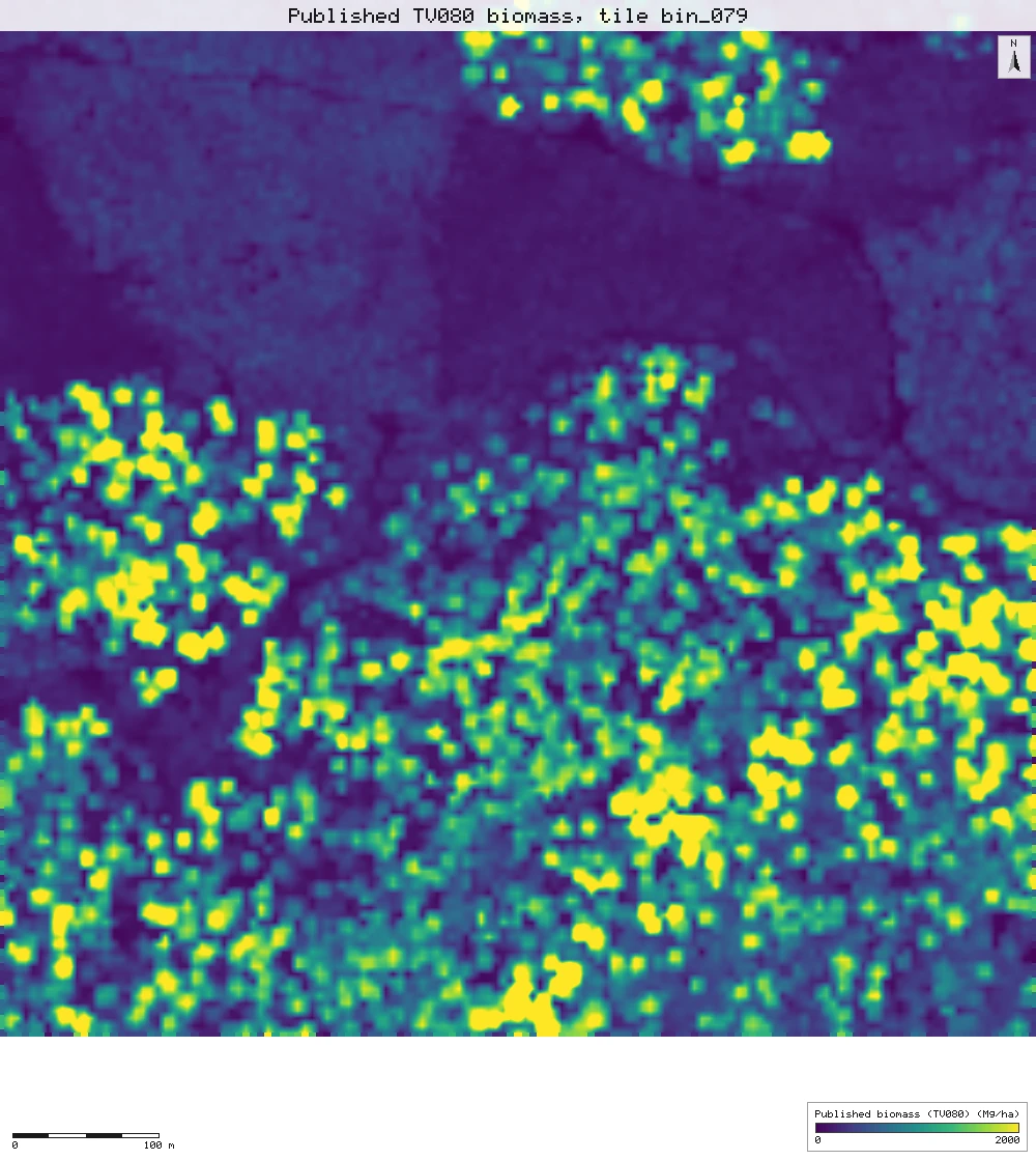
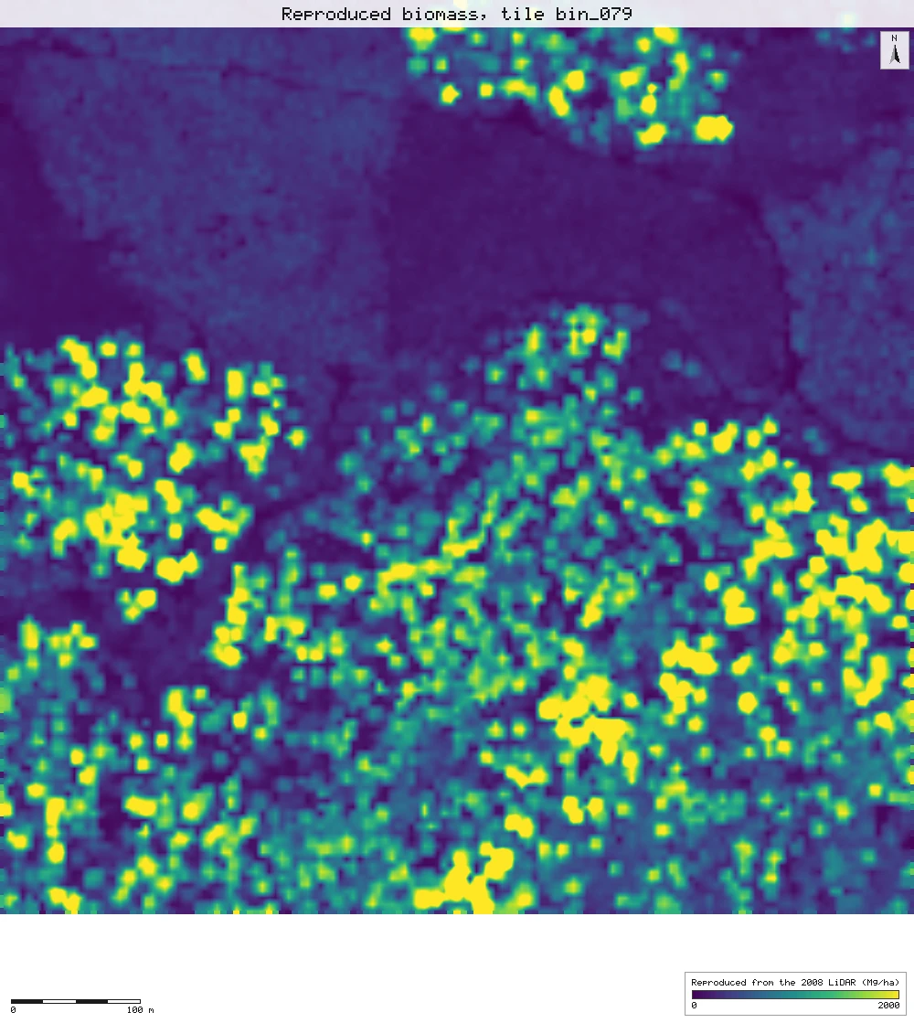
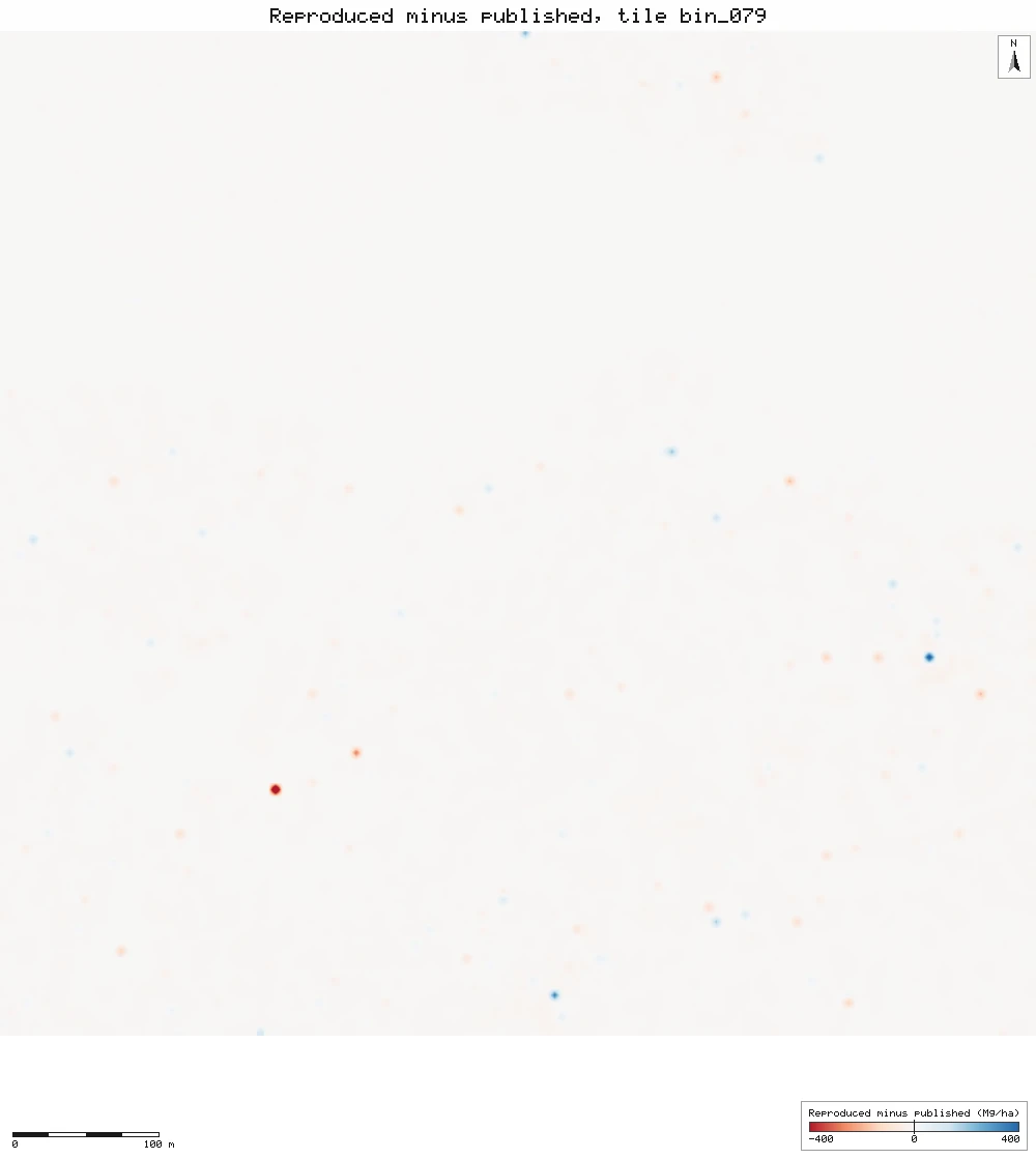
The middle tile, bin_079
The same 705 m square three ways: TV080 as published, our rebuild on TV080's own cells, and the difference (red: ours lower; blue: ours higher; colours stop at ±400 Mg/ha). The difference map is almost blank: nine cells in ten are within 12 Mg/ha.
Click or tap a map to open it full screen, then zoom and pan.
What was published
TV080 is a 5 m grid of aboveground live biomass in Mg/ha over the 2008 HJ Andrews LiDAR area, made with the equation of Seidl et al. (2012). Its metadata records the exact calculation: biomass = 400 × (0.1870714 + 0.02105491 H95 + 0.0001975951 elevation + 0.0001773864 SD²)³, where H95 is the 95th percentile first-return height in a 5 m cell, elevation is the 5 m bare earth, and SD is the standard deviation of H95 in the 7 × 7 cells (35 m) around the cell. The cubed term is biomass in Mg per 25 m² cell; × 400 turns it into Mg per hectare.
Seidl et al. 2012 (journal) · Seidl et al. 2012 (Forest Service full text) · TV080 metadata · HJ Andrews data catalogue
Published method. The paper fits the cube root of biomass on 708 field plots, grouped into 41 spatially independent groups, and reports coefficients rounded to three figures (Table 2) with a bootstrapped adjusted R² of 0.768. Old growth, as the paper delineates it (2,191 ha), averages 435.1 Mg C/ha of aboveground live carbon at a carbon content of 50%, which is 870.2 Mg/ha of biomass.
The data and where it came from
All of it is open: downloaded without an account or a form.
| Data | Where | Licence |
|---|---|---|
| TV080 biomass grid, tv08001.zip: tv08001.e00 (a 5 m integer grid in E00 export form, 2,872 × 2,154 cells, NAD83 UTM zone 10N) with FGDC metadata | HJ Andrews LTER, 6.8 MB zip (sha256 9e418923…c564de8b), downloaded without a form https://andrewsforest.oregonstate.edu/sites/default/files/lter/data/studies/spatialdata/tv08001.zip | Use constraints "no legal constraints", acknowledgement requested (HJ Andrews data policy, CC BY) |
| The 2008 LiDAR flight the grid was made from (Watershed Sciences, 10–11 August 2008): seven 750 × 750 m tiles, ot_HJ_Andrews_bin_029, 039, 054, 079, 110, 136 and 163, N 4897150–4897900, EPSG:26910 | OpenTopography OTLAS.082011.26910.1, anonymous bulk download (25 to 37 MB per tile) https://portal.opentopography.org/lidarDataset?opentopoID=OTLAS.082011.26910.1 | Treated as CC BY 4.0 with attribution to HJ Andrews / Watershed Sciences (HJ Andrews catalogue GI010); OpenTopography lists the licence as not provided |
| The flight's tile index (HJAnd_OR_TileIndex.shp), for the map | OpenTopography, same bulk folder https://opentopography.s3.sdsc.edu/pc-bulk/HJAnd_OR/HJAnd_OR_TileIndex.zip | As the LiDAR |
| HJ Andrews Experimental Forest boundary (GI006, boundary83.shp), for the map | HJ Andrews LTER, zip, no form or account https://andrewsforest.oregonstate.edu/sites/default/files/lter/data/studies/spatialdata/gi00601.zip | HJ Andrews data policy (CC BY, acknowledgement requested) |
The input files the run read, pinned by checksum
| File (relative to the data folder) | Bytes | sha256 |
|---|---|---|
samples/tv080/x/tv08001.e00 | 89,653,180 | b3b4f0a0a8229d9d… |
samples/ot2008/ot_HJ_Andrews_bin_029.laz | 24,955,073 | fdfda3f607e0b651… |
samples/ot2008/ot_HJ_Andrews_bin_039.laz | 27,163,073 | 8b14913fcf9010d4… |
samples/ot2008/ot_HJ_Andrews_bin_054.laz | 37,364,217 | fd78d0fd9171b8da… |
samples/ot2008/ot_HJ_Andrews_bin_079.laz | 30,167,254 | 92a1e0b5a89c15e1… |
samples/ot2008/ot_HJ_Andrews_bin_110.laz | 24,612,702 | f39e9fab0e97f5dc… |
samples/ot2008/ot_HJ_Andrews_bin_136.laz | 31,573,048 | b666e41d3daf2ead… |
samples/ot2008/ot_HJ_Andrews_bin_163.laz | 37,342,138 | 561ae324ea96e005… |
samples/ot2008idx/x/HJAnd_OR_TileIndex.shp | 25,804 | 9cdba01734e369e3… |
samples/hja-open/gi00601/x/boundary83.shp | 10,540 | 0774de0a9ebd9693… |
Full checksums are in run.json. Replay refuses an input whose checksum differs.
Method
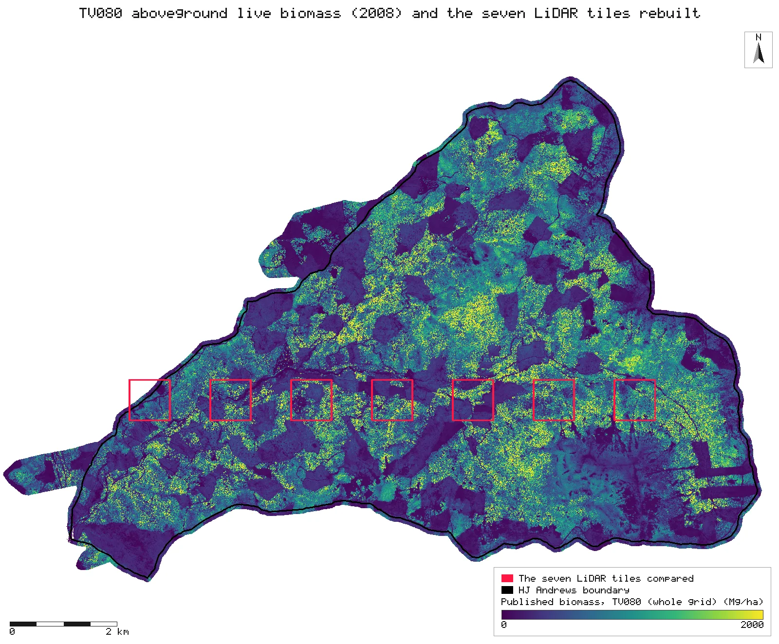
- Open the TV080 grid (E00) and the seven LiDAR tiles. The tiles are every second whole tile on one west-to-east row across the forest (N 4897150–4897900, from E 560100 to 569100), chosen by that rule before anything was compared.
- Per tile: LiDAR QA, then the ground classification delivered with the flight (gis_lidar_ground mode existing).
- Elevation: a 5 m TIN bare-earth grid (gis_lidar_dtm) on TV080's grid lines (align to the TV080 grid). Heights: normalised to a 1 m TIN bare earth.
- H95: the 95th percentile of first-return heights in each 5 m cell (gis_lidar_metrics, returns first, R type 7 percentile), on TV080's grid lines too, so each of our cells is the same 5 m square as a TV080 cell.
- SD: the population standard deviation of H95 over the 7 × 7 cells around each cell (gis_process focal).
- Biomass: the published equation with the published coefficients (gis_process calc). Nothing is fitted.
- Cut ours and TV080 to the same cells: every cell at least 20 m inside a tile edge, so the 35 m window never runs off its tile (gis_process calc with an extent on TV080's cell edges). No interpolation: the cells are the same.
- Compare with TV080 per tile and over all seven tiles as one surface (gis_compare surface with correlation): mean difference, MAE, RMSE, Pearson r and the least-squares line; the share of cells within 10% of the published value (gis_process calc).
- Render the maps: TV080 over the whole forest with the seven tiles outlined, and the middle tile (bin_079) published, reproduced and differenced.
The run made 155 NativeGIS calls: gis_open × 10, gis_lidar_qa × 7, gis_lidar_ground × 7, gis_lidar_dtm × 14, gis_lidar_metrics × 7, gis_close × 56, gis_process × 37, gis_compare × 8, gis_query × 1, gis_render × 8.
Published numbers next to ours
Seven LiDAR tiles against TV080
| LiDAR tile | West edge (E, m) | Cells compared | Mean difference (Mg/ha) | MAE (Mg/ha) | RMSE (Mg/ha) | r | Largest 7×7 SD of H95 (m) |
|---|---|---|---|---|---|---|---|
| bin_029 | 560,100 | 14,969 | −4.2 | 4.4 | 7.7 | 0.9999 | 22.1 |
| bin_039 | 561,600 | 19,881 | −4.7 | 5.2 | 14.9 | 0.9997 | 27.6 |
| bin_054 | 563,100 | 19,881 | −4.8 | 5.3 | 9.9 | 0.9999 | 27.1 |
| bin_079 | 564,600 | 19,881 | −4.9 | 5.5 | 11.7 | 0.9999 | 28.7 |
| bin_110 | 566,100 | 19,881 | −4.3 | 4.6 | 8.9 | 0.9999 | 27.1 |
| bin_136 | 567,600 | 19,881 | −5.8 | 6.5 | 15.7 | 0.9997 | 24.5 |
| bin_163 | 569,100 | 19,881 | −6.0 | 6.6 | 13.0 | 0.9998 | 27.2 |
| All seven | 134,255 | −5.0 | 5.5 | 12.1 | 0.9998 |
Per tile [22, 47, 72, 97, 122, 147, 173], all seven [183]. Difference = reproduced − published, cell for cell: our 5 m cells are TV080's cells (gis_lidar_dtm and gis_lidar_metrics aligned to the TV080 grid). r is Pearson's, from gis_compare. Tile bin_029 reaches past the forest boundary, where TV080 has no cells. Units: Mg of aboveground live biomass per hectare, 5 m cells, NAD83 / UTM zone 10N.
The seven tiles as one surface
| Published (TV080) | Reproduced | |
|---|---|---|
| Mean over the 134,255 cells (Mg/ha) | 637.4 | 632.5 |
| Standard deviation (Mg/ha) | 598.9 | 595.8 |
| Correlation, cell by cell (r) | 0.9998 | |
| Least-squares line, reproduced on published | -1.6 + 0.995 × published | |
| Difference: median, 5th to 95th percentile (Mg/ha) | −4.1; −11.9 to −0.9 | |
| Cells within 10% of the published value | 99.8% | |
| Before alignment (previous recording): RMSE, r | 161 Mg/ha, 0.97 | |
Means and standard deviations [182, 181]; r, the line and the difference percentiles [183]; within 10% [184]. Standard deviations are population moments. The before-alignment row is quoted from the previous recording (commit e6ce80f: our 5 m grid 1 m west and 1 m north of TV080's, sampled bilinearly at TV080's cell centres), not from this run.
Why any numbers differ
- The map is reproduced cell for cell. Over 134,255 cells (335.6 ha) the correlation with TV080 is 0.9998, the RMSE per 5 m cell is 12.1 Mg/ha and the MAE 5.5 Mg/ha, and 99.8% of cells are within 10% of the published value. Per tile the RMSE runs from 7.7 Mg/ha on bin_029, the tile with the least biomass, to 15.7 on bin_136, and r is 0.9997 or more on every tile.
- What is left is a small, steady shortfall. The reproduced mean is 632.5 Mg/ha against TV080's 637.4, 5.0 Mg/ha lower (−0.8%). The shortfall is nearly the same everywhere: every tile is between −6.0 and −4.2 Mg/ha, the median cell difference is −4.1 Mg/ha, and 90% of cells lie between −11.9 and −0.9 Mg/ha. The least-squares line, reproduced = −1.6 + 0.995 × published, says the same: about half a percent low across the whole range. A one-sided offset like this points to an input that differs slightly everywhere rather than to position; the candidates are below. It was not adjusted.
- Same cells, not 1 m apart. TV080's cell edges fall at easting 1 and northing 4 (modulo 5 m). This run builds the 5 m elevation and H95 grids on those lines (align to the TV080 grid), so each reproduced cell holds the same points as its TV080 cell. The previous recording of this study could not: its 5 m cells sat 1 m west and 1 m north of TV080's and were sampled bilinearly at TV080's cell centres, which gave the same mean (632.6 Mg/ha) but r 0.97, an RMSE of 161 Mg/ha and only 50% of cells within 10%. That scatter, red–blue pairs across the old forest, was the 1 m offset on a surface that changes sharply from crown to gap, not the method.
- What else can differ. The bare earth: TV080 used a 5 m bare-earth grid from the vendor's ground model; we use the ground points delivered with the flight, which are sparse. The percentile: the paper's LiDAR software may compute the 95th percentile with another interpolation rule or a minimum height, which neither the paper nor the metadata states. TV080 stores whole Mg/ha.
- The paper's own figures need data that is not public. The adjusted R² of 0.768 comes from 708 field plots that are not shared. The old-growth mean of 435.1 Mg C/ha (870.2 Mg/ha of biomass at 50% carbon) needs the paper's 2,191 ha old-growth delineation, which is not published either. For scale: TV080 as a whole averages 612.9 Mg/ha over 2,775,279 cells (6,938 ha), plantations included, and peaks at 5,144 Mg/ha.
- Small inconsistencies in the sources, none affecting the result. The paper says the LiDAR was flown in 2007; the data set's metadata says 10–11 August 2008. Table 2 prints the upper bound for H95 as 0.231, where the estimate is 0.0211. TV080's metadata spells the unit as milligrams per hectare; the values are megagrams (Mg/ha). Table 2 rounds the coefficients to three figures; TV080's lineage gives them in full, and those are the ones used here.
Replay it yourself
The run file records every call, its arguments, the checksums of the files it read and the numbers it returned. Replaying it repeats every call in a fresh NativeGIS session and checks that each answer comes out the same.
- Make an empty data folder and fetch the inputs into it exactly as below (bash; the folder layout is the one the run file expects):
cd /path/to/an/empty/folder
mkdir -p samples/tv080 && curl -fL -o samples/tv080/tv08001.zip https://andrewsforest.oregonstate.edu/sites/default/files/lter/data/studies/spatialdata/tv08001.zip && unzip -o samples/tv080/tv08001.zip -d samples/tv080/x
mkdir -p samples/ot2008 && curl -fL -o samples/ot2008/ot_HJ_Andrews_bin_029.laz https://opentopography.s3.sdsc.edu/pc-bulk/HJAnd_OR/ot_HJ_Andrews_bin_029.laz
mkdir -p samples/ot2008 && curl -fL -o samples/ot2008/ot_HJ_Andrews_bin_039.laz https://opentopography.s3.sdsc.edu/pc-bulk/HJAnd_OR/ot_HJ_Andrews_bin_039.laz
mkdir -p samples/ot2008 && curl -fL -o samples/ot2008/ot_HJ_Andrews_bin_054.laz https://opentopography.s3.sdsc.edu/pc-bulk/HJAnd_OR/ot_HJ_Andrews_bin_054.laz
mkdir -p samples/ot2008 && curl -fL -o samples/ot2008/ot_HJ_Andrews_bin_079.laz https://opentopography.s3.sdsc.edu/pc-bulk/HJAnd_OR/ot_HJ_Andrews_bin_079.laz
mkdir -p samples/ot2008 && curl -fL -o samples/ot2008/ot_HJ_Andrews_bin_110.laz https://opentopography.s3.sdsc.edu/pc-bulk/HJAnd_OR/ot_HJ_Andrews_bin_110.laz
mkdir -p samples/ot2008 && curl -fL -o samples/ot2008/ot_HJ_Andrews_bin_136.laz https://opentopography.s3.sdsc.edu/pc-bulk/HJAnd_OR/ot_HJ_Andrews_bin_136.laz
mkdir -p samples/ot2008 && curl -fL -o samples/ot2008/ot_HJ_Andrews_bin_163.laz https://opentopography.s3.sdsc.edu/pc-bulk/HJAnd_OR/ot_HJ_Andrews_bin_163.laz
mkdir -p samples/ot2008idx && curl -fL -o samples/ot2008idx/HJAnd_OR_TileIndex.zip https://opentopography.s3.sdsc.edu/pc-bulk/HJAnd_OR/HJAnd_OR_TileIndex.zip && unzip -o samples/ot2008idx/HJAnd_OR_TileIndex.zip -d samples/ot2008idx/x
mkdir -p samples/hja-open/gi00601 && curl -fL -o samples/hja-open/gi00601/gi00601.zip https://andrewsforest.oregonstate.edu/sites/default/files/lter/data/studies/spatialdata/gi00601.zip && unzip -o samples/hja-open/gi00601/gi00601.zip -d samples/hja-open/gi00601/x
- Download run.json (299,011 bytes, sha256
2e50bfe909f00c22eccab60a921bb6de17109fd6f4fcf2ff3f141285c68300aa). - Ask your assistant to replay it with NativeGIS, or call the tool directly:
gis_replay {"action": "replay",
            "file": "<absolute path to the run.json you downloaded>",
            "inputRoot": "<your data folder>",
            "outputRoot": "<a new, empty folder>"}
Paths in the run file are relative to the data folder (inputRoot), and outputs go under outputRoot, so nothing depends on where the original run lived.
Files
- run.json: the recorded run: every call, its arguments and the numbers it returned
Limits
- Seven tiles of 189, 335.6 ha of TV080's 6,938 ha, along one row across the middle of the forest. The tiles are processed one at a time and the 20 m edge strips are left out. gis_lidar_tiled now takes first-return 5 m metrics aligned to a template and joins tiles without seams, but these seven tiles are not neighbours, so its buffers would need tiles outside the set chosen in advance; the per-tile run is kept.
- The largest 7 × 7 SD of H95 in these tiles is 28.7 m, so a filter on high SD would not change any cell here.
- Nothing was tuned. The coefficients are the published ones, the tiles were picked by a rule before comparing, and the grid is TV080's own, taken as its file gives it.