NativeCAD · simulation coupling

A jet engine, solved: compressible CFD, combustion chemistry and a full start-up in one loop.

NativeCAD puts a fast engineering model at the centre of a design and wires real solvers around it. SU2 solves the compressible flow through the compressor and the exhaust nozzle, Cantera burns the fuel zone by zone, and the fast model runs the whole engine from starter to full power with their results built in. Every number traces back to the run that made it.

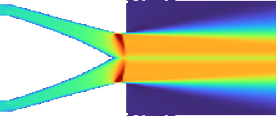
Mach-number field from the SU2 solution of the exhaust nozzle, mirrored about the engine axis: slow gas around the tail cone accelerating through the converging cone to a fast jet leaving the lip, with still air outside SU2 · compressible RANS · Mach number
0.00.51.01.3+ The built exhaust nozzle, solved: exit Mach 0.868 and 298.1 N of thrust against the 300 N target. How ↓
The coupling loop A fast model sits in the middle: the engine cycle, compressor and turbine maps, and the start-up run (thumbnail: shaft speed from starter to full power). Around it, Cantera (combustion chemistry, thumbnail: gas temperature through the combustor zones) and SU2 (compressible CFD, thumbnail: the nozzle Mach field) each calibrate it and check it. CalculiX (stress and vibration) checks parts and is next on this engine. CAD holds the real parts: the fast model sizes them, and the solvers run on their real shape. calibrate check calibrate check sizes the parts Fast model cycle · maps start-up run Cantera combustion chemistry SU2 compressible CFD CalculiX stress & vibration on our other parts CAD the real parts
calibrate: a solver measures a correction and the fast model is re-run with it check: a solver re-computes a result the fast model already gave dashed: done on other parts, next on this engine
0.86 → 0.965nozzle flow coefficient: what CFD measured on the first nozzle, then on the reshaped one
0.11 %compressor CFD against the fast model, mass flow at the design pressure ratio
1,098.5 Kcombustor exit from the chemistry solver, against a 1,100 K target
13.6 sfrom starter on to idle, simulated with the calibrated model

Compressible CFD: the exhaust nozzle

The nozzle is where the thrust comes from, so we solve it properly: SU2 8.5.0, compressible Reynolds-averaged Navier–Stokes with the Spalart–Allmaras turbulence model, axisymmetric, from the turbine exit out into the exhaust plume on 73,000 cells. The inlet is the cycle's own turbine-exit state, and the walls are the nozzle and tail cone the parts are built to.

0.598 kg/smass flow, cycle 0.594 kg/s
0.868exit Mach, area-averaged (0.665 on the axis)
298.1 Nthrust, against a 300 N target
0.982total pressure kept through the nozzle

The field at the top of this page is that solution. Gas arrives as an annular jet along the outer wall, closes in behind the tail cone and accelerates through the 15° cone to about 500 m/s at the exit. It leaves the lip still converging, and that is where the flow deficit sits rather than in a pressure loss: the nozzle keeps 98.2 % of its total pressure. A fast model cannot see that; the CFD can, and it is what reshaped this nozzle (step 4 below).

Compressible CFD: transonic flow on the compressor blades

SU2 also solves the compressor: one passage of the 12-blade impeller in the rotating frame, 47,040 cells, at 6 back pressures. That traces the impeller's speed line from a pressure ratio of 2.95 to 4.30. At the design pressure ratio of 3.5 the CFD passes 0.584 kg/s against the cycle's 0.583. On the blades the flow goes supersonic: the suction-side Mach number peaks at 1.19 at mid-span and 1.39 near the tip.

3.03.54.0 0.560.570.58 mass flow (kg/s) total pressure ratio cycle 0.583 kg/s mass flow (kg/s) 0.553, total pressure ratio 4.297mass flow (kg/s) 0.565, total pressure ratio 4.127mass flow (kg/s) 0.573, total pressure ratio 3.959mass flow (kg/s) 0.582, total pressure ratio 3.611mass flow (kg/s) 0.586, total pressure ratio 3.282mass flow (kg/s) 0.587, total pressure ratio 2.947 design point, PR 3.50 CFD speedline
7580859095 0.560.570.58 mass flow (kg/s) efficiency (%) cycle 0.583 kg/s mass flow (kg/s) 0.553, efficiency (%) 93.824mass flow (kg/s) 0.565, efficiency (%) 92.419mass flow (kg/s) 0.573, efficiency (%) 90.217mass flow (kg/s) 0.582, efficiency (%) 85.236mass flow (kg/s) 0.586, efficiency (%) 80.027mass flow (kg/s) 0.587, efficiency (%) 73.459 isentropic efficiency
0.00.51.0 0.00.51.0 normalised chord, 50 % span isentropic Mach normalised chord, 50 % span 0.000, isentropic Mach 0.592normalised chord, 50 % span 0.010, isentropic Mach 0.685normalised chord, 50 % span 0.021, isentropic Mach 0.765normalised chord, 50 % span 0.032, isentropic Mach 0.810normalised chord, 50 % span 0.044, isentropic Mach 0.836normalised chord, 50 % span 0.056, isentropic Mach 0.859normalised chord, 50 % span 0.069, isentropic Mach 0.890normalised chord, 50 % span 0.083, isentropic Mach 0.936normalised chord, 50 % span 0.097, isentropic Mach 0.982normalised chord, 50 % span 0.112, isentropic Mach 1.018normalised chord, 50 % span 0.128, isentropic Mach 1.061normalised chord, 50 % span 0.144, isentropic Mach 1.109normalised chord, 50 % span 0.161, isentropic Mach 1.153normalised chord, 50 % span 0.178, isentropic Mach 1.183normalised chord, 50 % span 0.197, isentropic Mach 1.188normalised chord, 50 % span 0.215, isentropic Mach 1.167normalised chord, 50 % span 0.235, isentropic Mach 1.136normalised chord, 50 % span 0.255, isentropic Mach 1.112normalised chord, 50 % span 0.275, isentropic Mach 1.101normalised chord, 50 % span 0.296, isentropic Mach 1.102normalised chord, 50 % span 0.317, isentropic Mach 1.112normalised chord, 50 % span 0.339, isentropic Mach 1.128normalised chord, 50 % span 0.361, isentropic Mach 1.146normalised chord, 50 % span 0.384, isentropic Mach 1.165normalised chord, 50 % span 0.407, isentropic Mach 1.181normalised chord, 50 % span 0.430, isentropic Mach 1.188normalised chord, 50 % span 0.453, isentropic Mach 1.182normalised chord, 50 % span 0.477, isentropic Mach 1.160normalised chord, 50 % span 0.500, isentropic Mach 1.114normalised chord, 50 % span 0.523, isentropic Mach 1.024normalised chord, 50 % span 0.547, isentropic Mach 0.964normalised chord, 50 % span 0.570, isentropic Mach 0.996normalised chord, 50 % span 0.593, isentropic Mach 1.058normalised chord, 50 % span 0.616, isentropic Mach 1.099normalised chord, 50 % span 0.639, isentropic Mach 1.117normalised chord, 50 % span 0.661, isentropic Mach 1.123normalised chord, 50 % span 0.683, isentropic Mach 1.124normalised chord, 50 % span 0.704, isentropic Mach 1.126normalised chord, 50 % span 0.725, isentropic Mach 1.130normalised chord, 50 % span 0.745, isentropic Mach 1.137normalised chord, 50 % span 0.765, isentropic Mach 1.143normalised chord, 50 % span 0.785, isentropic Mach 1.149normalised chord, 50 % span 0.803, isentropic Mach 1.157normalised chord, 50 % span 0.822, isentropic Mach 1.157normalised chord, 50 % span 0.839, isentropic Mach 1.149normalised chord, 50 % span 0.856, isentropic Mach 1.140normalised chord, 50 % span 0.872, isentropic Mach 1.131normalised chord, 50 % span 0.888, isentropic Mach 1.121normalised chord, 50 % span 0.903, isentropic Mach 1.110normalised chord, 50 % span 0.917, isentropic Mach 1.098normalised chord, 50 % span 0.931, isentropic Mach 1.086normalised chord, 50 % span 0.944, isentropic Mach 1.074normalised chord, 50 % span 0.956, isentropic Mach 1.063normalised chord, 50 % span 0.968, isentropic Mach 1.053normalised chord, 50 % span 0.979, isentropic Mach 1.039normalised chord, 50 % span 0.990, isentropic Mach 1.047normalised chord, 50 % span 1.000, isentropic Mach 1.115 suction side
0.00.51.0 0.00.51.0 normalised chord, 90 % span isentropic Mach normalised chord, 90 % span 0.000, isentropic Mach 0.750normalised chord, 90 % span 0.010, isentropic Mach 0.816normalised chord, 90 % span 0.021, isentropic Mach 0.887normalised chord, 90 % span 0.032, isentropic Mach 0.945normalised chord, 90 % span 0.044, isentropic Mach 0.991normalised chord, 90 % span 0.056, isentropic Mach 1.030normalised chord, 90 % span 0.069, isentropic Mach 1.065normalised chord, 90 % span 0.083, isentropic Mach 1.104normalised chord, 90 % span 0.097, isentropic Mach 1.138normalised chord, 90 % span 0.112, isentropic Mach 1.166normalised chord, 90 % span 0.128, isentropic Mach 1.205normalised chord, 90 % span 0.144, isentropic Mach 1.263normalised chord, 90 % span 0.161, isentropic Mach 1.332normalised chord, 90 % span 0.178, isentropic Mach 1.385normalised chord, 90 % span 0.197, isentropic Mach 1.374normalised chord, 90 % span 0.215, isentropic Mach 1.299normalised chord, 90 % span 0.235, isentropic Mach 1.238normalised chord, 90 % span 0.255, isentropic Mach 1.219normalised chord, 90 % span 0.275, isentropic Mach 1.219normalised chord, 90 % span 0.296, isentropic Mach 1.216normalised chord, 90 % span 0.317, isentropic Mach 1.209normalised chord, 90 % span 0.339, isentropic Mach 1.202normalised chord, 90 % span 0.361, isentropic Mach 1.198normalised chord, 90 % span 0.384, isentropic Mach 1.188normalised chord, 90 % span 0.407, isentropic Mach 1.173normalised chord, 90 % span 0.430, isentropic Mach 1.155normalised chord, 90 % span 0.453, isentropic Mach 1.134normalised chord, 90 % span 0.477, isentropic Mach 1.111normalised chord, 90 % span 0.500, isentropic Mach 1.092normalised chord, 90 % span 0.523, isentropic Mach 1.078normalised chord, 90 % span 0.547, isentropic Mach 1.071normalised chord, 90 % span 0.570, isentropic Mach 1.070normalised chord, 90 % span 0.593, isentropic Mach 1.073normalised chord, 90 % span 0.616, isentropic Mach 1.081normalised chord, 90 % span 0.639, isentropic Mach 1.091normalised chord, 90 % span 0.661, isentropic Mach 1.102normalised chord, 90 % span 0.683, isentropic Mach 1.113normalised chord, 90 % span 0.704, isentropic Mach 1.124normalised chord, 90 % span 0.725, isentropic Mach 1.134normalised chord, 90 % span 0.745, isentropic Mach 1.142normalised chord, 90 % span 0.765, isentropic Mach 1.148normalised chord, 90 % span 0.785, isentropic Mach 1.151normalised chord, 90 % span 0.803, isentropic Mach 1.153normalised chord, 90 % span 0.822, isentropic Mach 1.149normalised chord, 90 % span 0.839, isentropic Mach 1.139normalised chord, 90 % span 0.856, isentropic Mach 1.129normalised chord, 90 % span 0.872, isentropic Mach 1.119normalised chord, 90 % span 0.888, isentropic Mach 1.108normalised chord, 90 % span 0.903, isentropic Mach 1.097normalised chord, 90 % span 0.917, isentropic Mach 1.085normalised chord, 90 % span 0.931, isentropic Mach 1.074normalised chord, 90 % span 0.944, isentropic Mach 1.063normalised chord, 90 % span 0.956, isentropic Mach 1.054normalised chord, 90 % span 0.968, isentropic Mach 1.044normalised chord, 90 % span 0.979, isentropic Mach 1.026normalised chord, 90 % span 0.990, isentropic Mach 1.024normalised chord, 90 % span 1.000, isentropic Mach 1.104 suction side

Speed line and efficiency from the 6 back pressures. Blade-surface Mach from the wall pressure on the suction side, at the back pressure nearest the design pressure ratio. The passage is meshed without a tip gap, so the efficiency reads on the high side.

Combustion chemistry, zone by zone

Cantera 3.2.0 models the combustor as a network of reactors with the GRI-Mech 3.0 mechanism and a jet-fuel surrogate: two stirred reactors where the flame sits, then two flow reactors where the rest of the air mixes in. Each strip below is the gas leaving one zone.

99.8 %combustion efficiency
2,337 Khottest zone, cooled to the turbine's limit by the dilution air
219 ppmCO at design, dry, 15 % O2
12 of 12throttle points where the network and the blowout screen agree

Will it stay lit?

Along the throttle line a lean-blowout screen and the reactor network both rate the flame. The sized liner stays lit all the way down to 45 % throttle, with a margin of 0.31 on the screen and 96 % in the network. As a control, a deliberately half-size liner goes through the same screen and blows out below 60 % throttle: the screen catches a bad design.

-0.50-0.250.000.250.500.751.000.50.60.70.80.91.0throttle (fraction of design mass flow)LBO margin Sized liner, throttle 0.45: LBO margin 0.3051Sized liner, throttle 0.5: LBO margin 0.3779Sized liner, throttle 0.55: LBO margin 0.4514Sized liner, throttle 0.6: LBO margin 0.5215Sized liner, throttle 0.65: LBO margin 0.5862Sized liner, throttle 0.7: LBO margin 0.6442Sized liner, throttle 0.75: LBO margin 0.6953Sized liner, throttle 0.8: LBO margin 0.7397Sized liner, throttle 0.85: LBO margin 0.778Sized liner, throttle 0.9: LBO margin 0.8108Sized liner, throttle 0.95: LBO margin 0.8387Sized liner, throttle 1: LBO margin 0.8624Half-size liner, throttle 0.45: LBO margin -0.3898 (blowout predicted)Half-size liner, throttle 0.5: LBO margin -0.2441 (blowout predicted)Half-size liner, throttle 0.55: LBO margin -0.0972 (blowout predicted)Half-size liner, throttle 0.6: LBO margin 0.0431Half-size liner, throttle 0.65: LBO margin 0.1723Half-size liner, throttle 0.7: LBO margin 0.2883Half-size liner, throttle 0.75: LBO margin 0.3906Half-size liner, throttle 0.8: LBO margin 0.4795Half-size liner, throttle 0.85: LBO margin 0.5561Half-size liner, throttle 0.9: LBO margin 0.6216Half-size liner, throttle 0.95: LBO margin 0.6775Half-size liner, throttle 1: LBO margin 0.7249Cantera network, throttle 0.45: LBO margin 0.9552Cantera network, throttle 0.5: LBO margin 0.9584Cantera network, throttle 0.55: LBO margin 0.9618Cantera network, throttle 0.6: LBO margin 0.9652Cantera network, throttle 0.65: LBO margin 0.9684Cantera network, throttle 0.7: LBO margin 0.9715Cantera network, throttle 0.75: LBO margin 0.9744Cantera network, throttle 0.8: LBO margin 0.977Cantera network, throttle 0.85: LBO margin 0.9793Cantera network, throttle 0.9: LBO margin 0.9815Cantera network, throttle 0.95: LBO margin 0.9834Cantera network, throttle 1: LBO margin 0.9851 blowout below this line

Sized liner (Lefebvre)Half-size liner (Lefebvre)Cantera network, sized liner

LBO margin is 1 minus the ratio of blowout loading to actual loading, one scale for every line: zero is blowout, above zero is stable.

How the solvers feed each other

Our worked example is a small jet engine: 300 N of thrust, a compressor turning at 64,213 rpm and a turbine inlet at 1,100 K. Every part is a real solid in NativeCAD. The fast model does the design in a blink; the solvers calibrate it (measure a correction and feed it back as a plain number) or check it (re-compute a result it already gave). When a correction changes the shape, the loop runs again.

  1. The fast model sizes the engine

    The engine cycle works out the air flow (0.583 kg/s), the temperatures and pressures at every station, and the size of every passage. NativeCAD builds the parts from those sizes.

  2. SU2 checks the compressor

    Quick blade-row estimates give the compressor and turbine maps. Compressible CFD on the impeller checks them: 6 points along its speed line, and at the design pressure ratio the simulated air flow lands 0.11 % from the model (the limit was 5 %).

  3. Cantera calibrates the burner, then checks it

    The chemistry solver worked out how hot jet fuel burns over 3,321 combinations of inlet temperature, pressure and fuel-to-air ratio. That table now sets how much fuel the fast model burns. Then a separate chemistry run models the combustor itself as 4 zones and checks the result: 1,098.5 K at the exit against the 1,100 K target, 0.13 % off, inside the 2 % limit.

  4. SU2 calibrates the nozzle

    The first SU2 run on the first nozzle found it let through less gas than the model assumed: a flow coefficient (Cd) of 0.86 where the model had 1.00, so 262 N of thrust instead of 300 and 12.8 % too little gas.

    So we reshaped it, with a 15° cone and a short straight lip at the exit, and sized the opening for a Cd of 0.97: 2,916 mm² instead of 2,829. The re-run measured 0.965 and 298.1 N, 0.6 % off the target. Each run took 34 and 64 minutes, which is exactly why the solver sits outside the fast model.

  5. The start-up, with everything calibrated

    With the burner and nozzle calibrated, the fast model plays a full start: starter, light-off at 2.9 s, idle at 13.6 s, full power 11.5 s later. The turbine never sees more than 1,100 K and the compressor keeps at least 26 % margin from stall. The energy books balance to 0.065 %.

Watch it start

The real engine, cut open, running the start-up above. Gas is coloured by temperature, the flame by the chemistry solver's zones, the jet by the airflow simulation. Turn and move the cut, orbit and zoom.

Loading the start-up run…
Simulated from the cycle and CFD results
0.0 s
View settings
–rpm
–exhaust gas temperature
–thrust
–fuel flow

▬ rpm  ▬ EGT  ·  particles coloured by gas temperature, 300 K2,400 K

Every number can be traced

A record for every correction

Each correction stores its value, its unit, the solver and version, the run, the inputs and a fingerprint of the result file. Replay the record and the whole loop re-runs without a single solver, to the same answer.

Pass marks set before the run

Every solver check has its acceptance limit fixed before the first run, and limits never move to fit a result.

Nobody grades their own work

The code that grades a result may not share code with the code that made it, and a test enforces that.

Limits today: the cad_couple tool is in the NativeCAD release and runs this loop, with Cantera and SU2 as calibrators, a run record with a content hash, and a replay that needs no solver. The coupling covers scalar correction factors only. Blade-row CFD and conjugate heat transfer (gas and metal temperatures solved together) are not part of it: the compressor and turbine maps are meanline correlations, and the metal temperature is not solved with the gas.

Bring us a problem

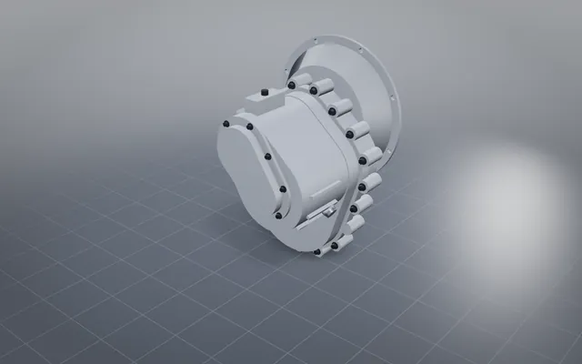
The pattern is not about jet engines. A fast model of your product in the middle, the right solver for each question around it, and a record behind every number. We have built pieces of it for all of these:

Pumps and turbopumps, pressure vessels, rocket engines, robot arms: if it can be modelled fast and checked by a solver, we can wire the loop. Tell us what you want built.

Tell us what you want built

NativeCAD runs inside your AI assistant. Bring a part, a product or a problem, and we will build the loop around it.
More demos

All demos →

Build your own part with NativeCAD

Free for education and makers with a registered key · $200 per seat per year · Kernel SDK for products.